Automatic Differentiation

Topics in Digital Heritage:
Numerical Methods for Digital Reconstruction

Jin Woo Lee

KAIST

Fall 2026

Recap

From Last Class: Finite Differences Hit a Floor

Finite differences approximate \(f'\) from samples:

\[ f'(x)\approx\frac{f(x+h)-f(x-h)}{2h} \]

Three problems remained:

1. An accuracy floor. Truncation error falls with \(h\), rounding error grows like \(\varepsilon/h\). We lose 5 to 8 of our 16 digits.
2. A step size to tune. The best \(h\) depends on the function and on the noise.
3. Cost grows with the number of inputs. The gradient of \(f:\mathbb{R}^n\to\mathbb{R}\) needs \(n+1\) evaluations of \(f\).

hs = np.logspace(-16, 0, 400)
x = torch.tensor(x0, requires_grad=True)
torch.sin(x**2).backward()                                 # automatic differentiation with PyTorch
ad_err = abs(x.grad.item() - df_test(x0))

fig, ax = plt.subplots(figsize=(5.2, 4.2))
for name, rule, col in [("forward difference", forward, "steelblue"), ("centered difference", centered, "forestgreen")]:
    err = np.array([abs(rule(f_test, x0, h) - df_test(x0)) for h in hs])
    ax.loglog(hs, np.maximum(err, 1e-17), color=col, lw=1, label=name)
ax.loglog(hs, eps / hs, color="k", ls="--", lw=1, label="rounding: $\\varepsilon/h$")
ax.axhline(max(ad_err, eps), color="firebrick", lw=2.5, label="automatic differentiation")
ax.text(1e-15, 4 * eps, f"error {ad_err:.1e}, no $h$ at all", color="firebrick", fontsize=8)
ax.set_ylim(1e-17, 10)
ax.set_xlabel("step size $h$"); ax.set_ylabel("|error| of $f'(1)$")
ax.set_title("$f(x)=\\sin x^2$: the error curve of last class", fontsize=9)
ax.legend(fontsize=7, loc="upper center")
plt.tight_layout()
plt.show()

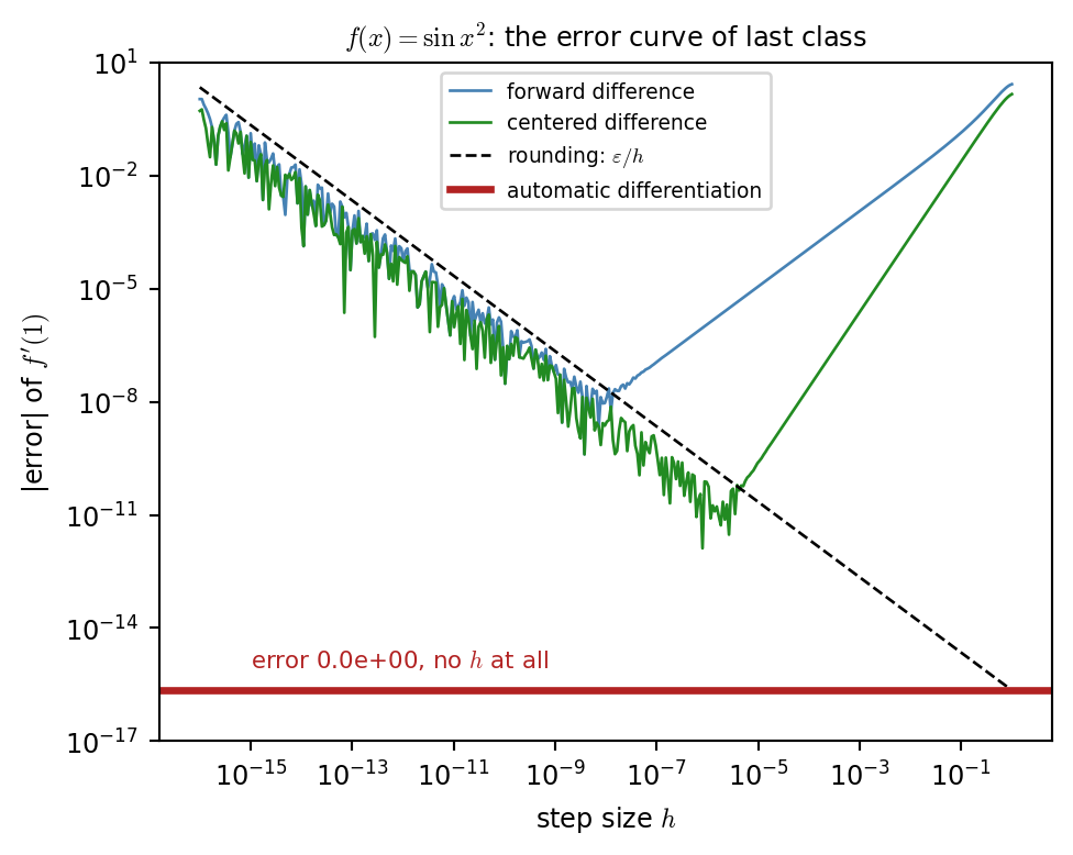
Today: differentiate the program that computes \(f\).

Three Ways to Get a Derivative

	By hand / symbolic	Finite differences	Automatic differentiation
Differentiates	a formula	a black box, or samples	a program
Result	a new formula	a number	a number
Error	none	truncation \(+\) rounding	rounding only
Cost for \(\nabla f\), \(n\) inputs	grows with the formula	\(n+1\) evaluations	about \(n\) (forward) or a few (reverse) evaluations
The catch	formulas explode; redo for every change of the model	step size, noise amplification	needs the source code; reverse mode needs memory

The idea. Every program is a sequence of elementary operations, and we know the derivative of each one. Chain them.

def f(x):
    v = x * x        # dv/dx = 2x
    y = sin(v)       # dy/dv = cos(v)
    return y         # dy/dx = cos(v) * 2x

Which one should I use?

• I have code for \(f\) (a simulation, a renderer, a network): automatic differentiation.
• I only have measured samples (a scan, a recording): finite differences on smoothed data, as in the last class.
• I want to verify my derivative: compare both.

Today’s ILO

• Describe what a computer does to get df/dx from a program f(x): record a tape, then walk it backward. Recognize backpropagation as the same algorithm.
• Explain how a physics-informed neural network turns a PDE into a loss, and evaluate it against finite differences.
• List other autodiff-based methods for science (neural ODEs, solver in the loop, neural operators, differentiable rendering and sound).

Autodiff and Backpropagation

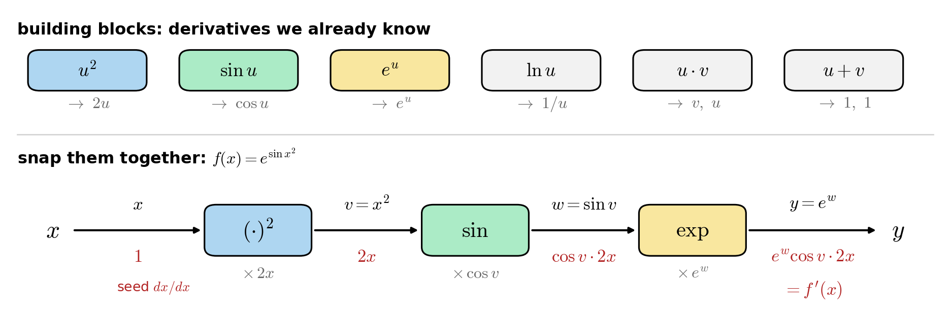
Snap Known Derivatives Together

\[ f(x)=\exp\big(\overbrace{\sin(\underbrace{x^2}_{v})}^{w}\big) \quad \Longrightarrow\quad f\,'(x)=\exp'(w)\cdot\sin'(v)\cdot(x^2)' =\color{firebrick}{e^{w}\cdot\cos v\cdot 2x}, \]

• Only each block’s derivative is needed, and we know it exactly: no \(h\), only rounding error.
• Forward mode carries \([\text{value},\ \text{derivative}]\) through the program; overloading *, +, sin leaves the code unchanged.
• A simulation is a long chain of blocks: exact for the program, numerical errors included, not for the physics.

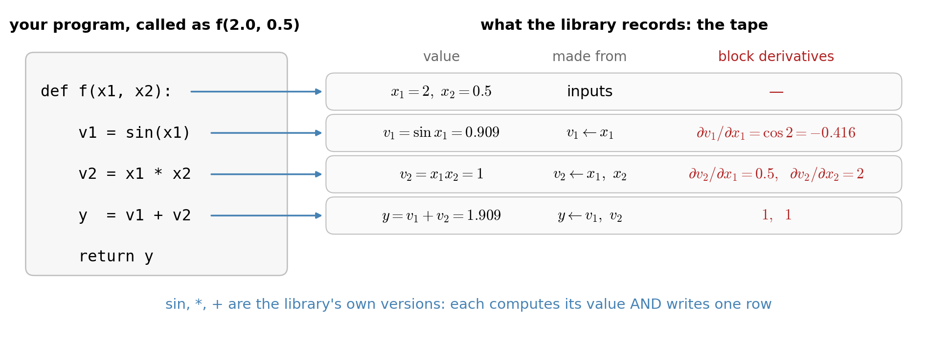
Calling f(x): The Library Writes a Tape

• The inputs are not plain floats but tracked numbers (a PyTorch or JAX tensor). Inside f, the operations sin, *, + are the library’s versions (not the plain Python operator.)
• Each operation does two things: return its value, and append one row to a list in memory, the tape. Drawn as arrows, the “made from” column is the computational graph.
• Nothing has been differentiated yet. Only block derivatives, evaluated at today’s numbers, are stored.

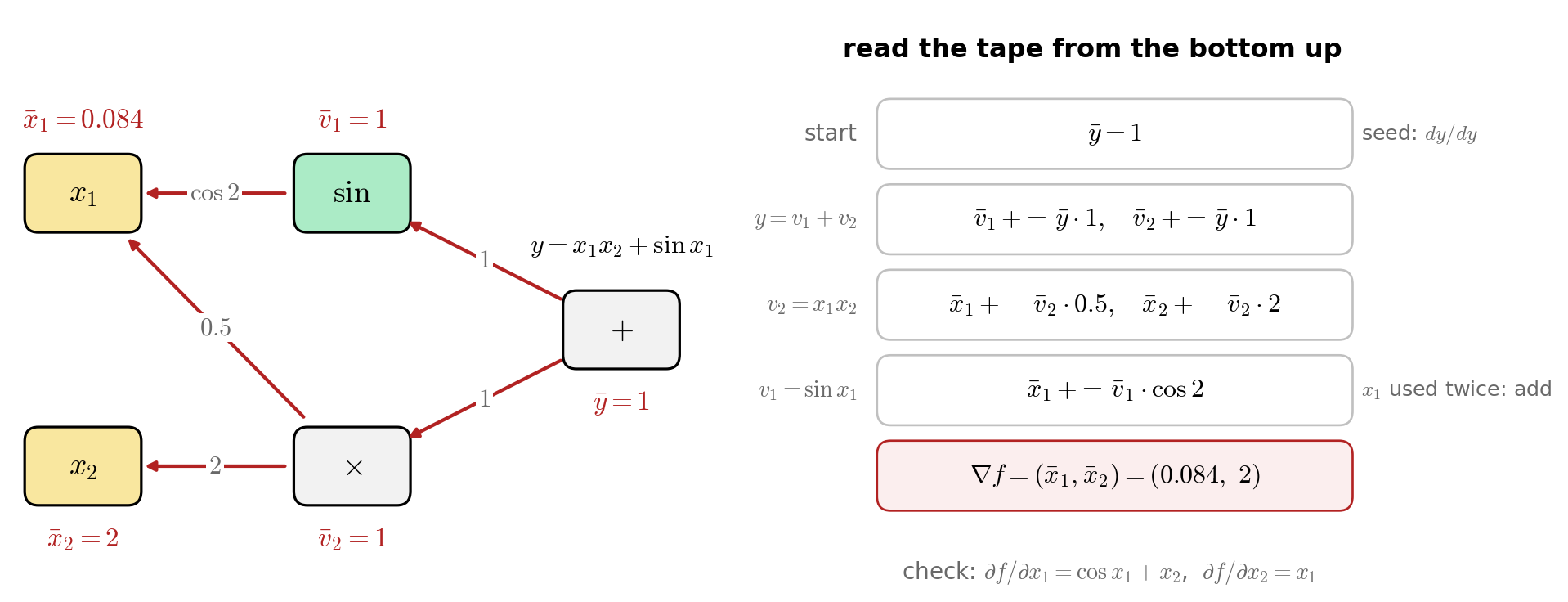
Then It Walks the Tape Backward

What the computer does to get df/dx from a program f(x)

1. Run f(x) on tracked inputs.
2. Seed the output: \(\bar y=1\) (the adjoint of the output with respect to itself).
3. Read the tape bottom up: \(\ \bar v_{\text{parent}}\ {+}{=}\ \bar v\cdot(\text{block derivative})\).
4. The adjoints of the inputs are \(\nabla f\): all inputs at once, for a few runs of f, holding the whole tape in memory.

cf. adjoint: \(\bar v\) is the derivative of the output with respect to \(v\), not the other way around. The adjoint of a block is the transpose of its Jacobian.

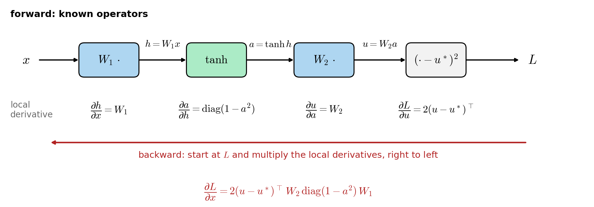
Backpropagation Is Reverse Mode on a Network

• A network is a program of known operators. Values are vectors, so each local derivative is a Jacobian
  • Backward pass through the chain rule
• Weight gradients come out on the way \[\partial L/\partial W_2=\bar u\,a^{\top},\qquad \partial L/\partial W_1=\bar h\,x^{\top}\]

• Computing derivatives requires holding the tape
  • Forward pass must store all intermediate values.
• Backpropagation (Rumelhart, Hinton & Williams, 1986) is reverse-mode autodiff (Linnainmaa, 1970) applied to a loss.

Autodiff for PDEs: Physics-Informed Networks

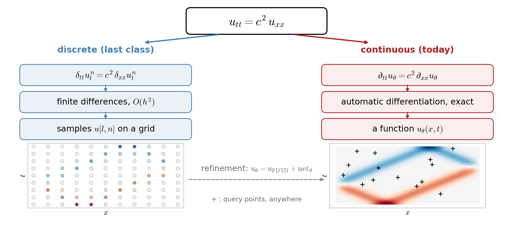
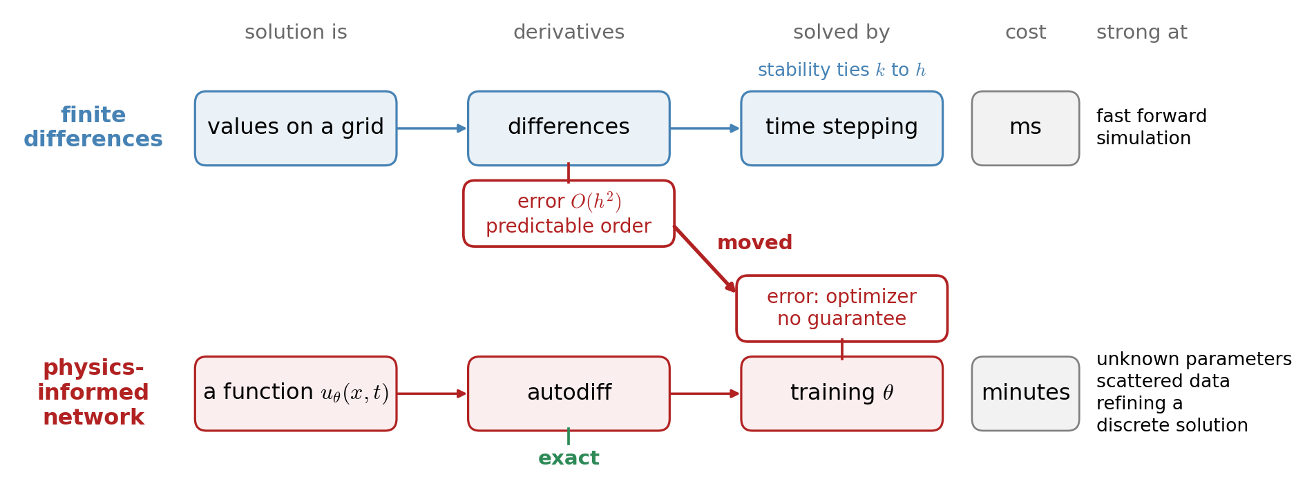
Two Ways to Differentiate a Wave Equation

Discrete: the solution is an array. Derivatives are differences with error \(O(h^2)\), and stability ties the time step to the grid spacing.

Continuous: the solution is a function \(u_\theta(x,t)\), here a neural network. Its derivatives are exact at any point, with no grid.

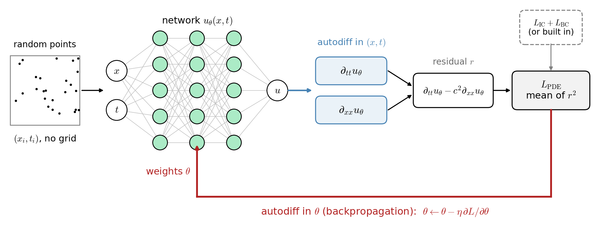
PINN: The Loss Is the Equation

\[ L(\theta)=L_{\text{PDE}}+L_{\text{IC}}+L_{\text{BC}},\qquad L_{\text{PDE}}=\frac1N\sum_{i=1}^N r(x_i,t_i)^2 \]

\[ r=\partial_{tt}u_\theta-c^2\,\partial_{xx}u_\theta \]

No recorded data, no reference solution, totally unsupervised.

We cannot write down the solution, but we can grade it.

Initial and Boundary Conditions

Today the conditions are built in:

\[ u_\theta(x,t)=u_0(x)+t^2\,x(1-x)\,\mathrm{net}_\theta(x,t) \]

so \(u_\theta=u_0\), \(\partial_tu_\theta=0\) at \(t=0\), and \(u_\theta=0\) at both ends.

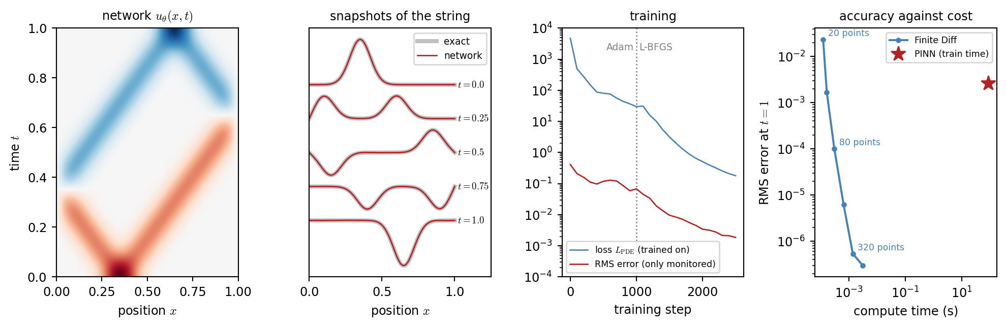
Result: A Plucked String Without a Grid

• Evaluate the performance critically. Single precision with Adam alone stalled near an RMS error of 0.2.
  • It took double precision, L-BFGS, and Fourier features to actually make PINN converge.
• For this forward problem, finite differences are far cheaper and their error is predictable.

Trade-offs: Where the Error Goes

The error did not disappear. It moved from the derivative to the optimizer.

The cost moved from milliseconds to minutes.

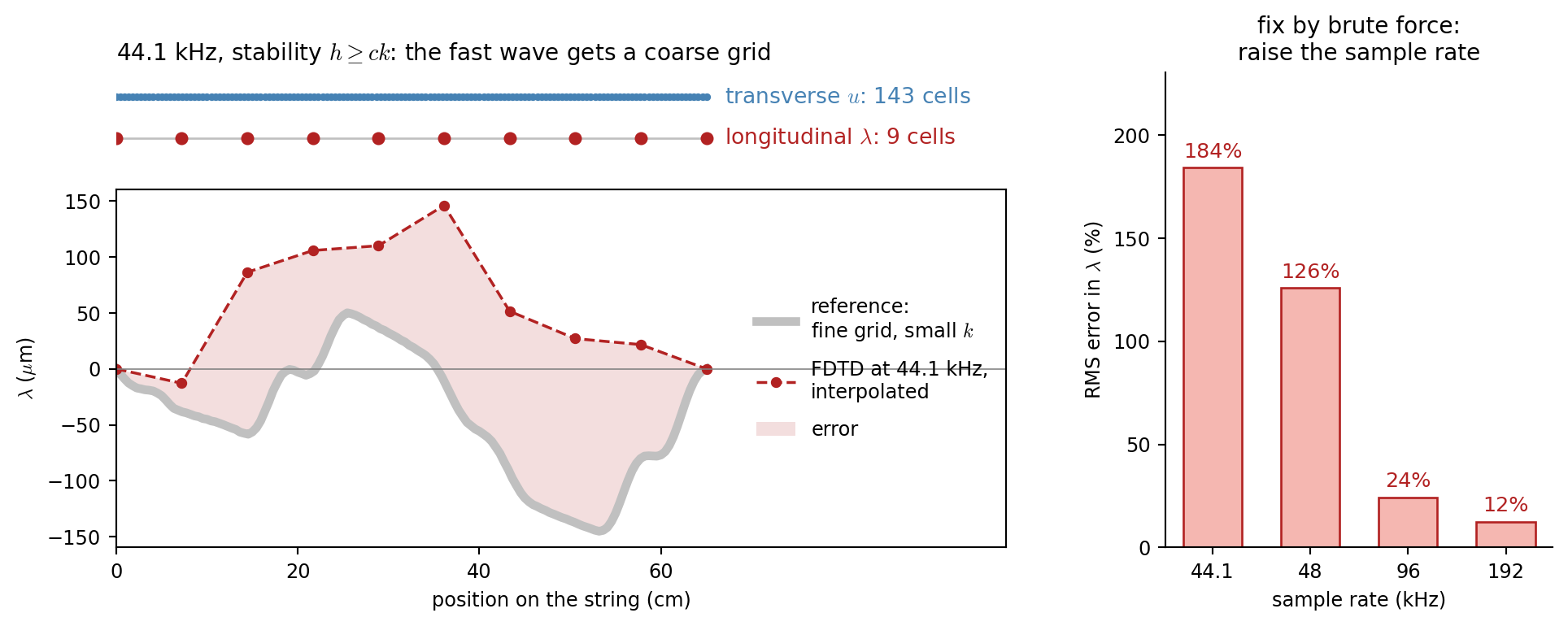
The Best of Both: Refining a String Simulation

Problem. At a fixed audio rate, stability \(h\ge ck\) gives the fast longitudinal wave a coarse grid. Coupling it to the transverse wave needs interpolation, which adds error.

Fix. Keep the FDTD solution and learn only a correction, \(\ u_\theta=u_{\text{FDTD}}+\mathrm{net}_\theta(x,t)\), trained with \(L_{\text{PDE}}\) alone: no ground truth.

Beyond PINNs: Autodiff in Scientific Machine Learning

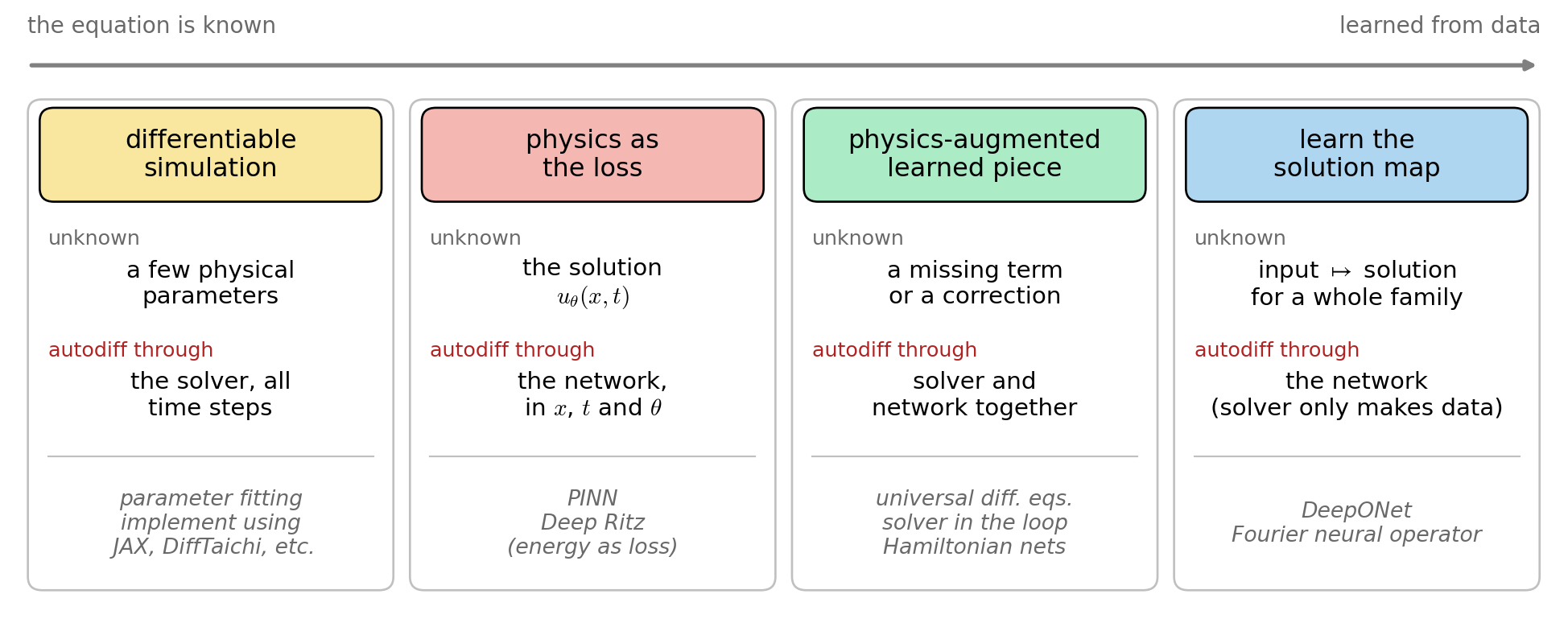
A Map of Approaches

Physics-augmented Learned Piece

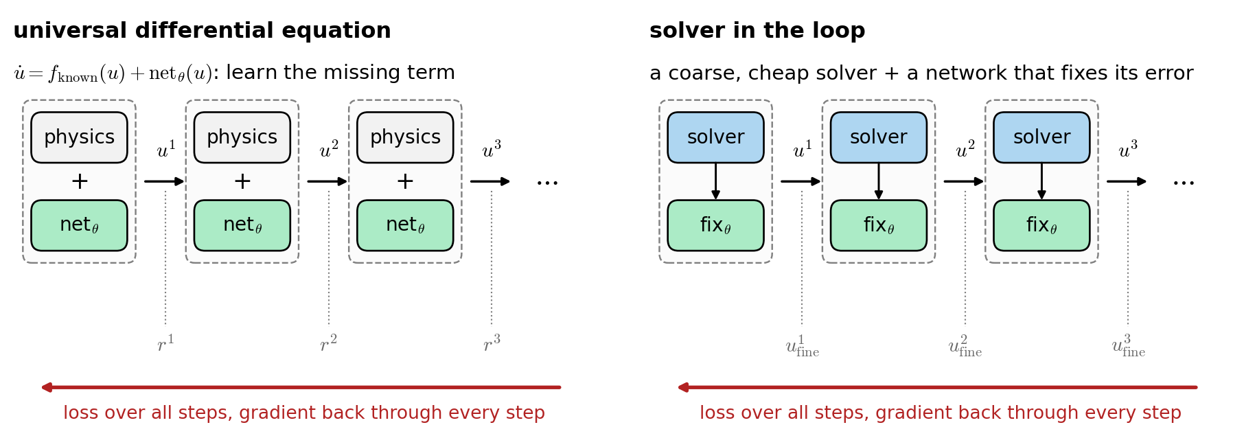
• Keep the physics you trust; a network learns only the missing term (a nonlinearity, a loss mechanism).
• Gradients through the solver, or by the adjoint method: a neural ODE when the whole right-hand side is a network.
• The learned term can be inspected, even distilled back into a formula by sparse regression.

• A coarse, cheap solver runs; a network corrects each step toward a fine reference.
• Training unrolls several steps, so the network sees the effect of its own corrections.
• The string refinement of the previous section is a cousin: the PDE residual replaces the fine reference.

cf. solver-in-the-loop for fluid simulation

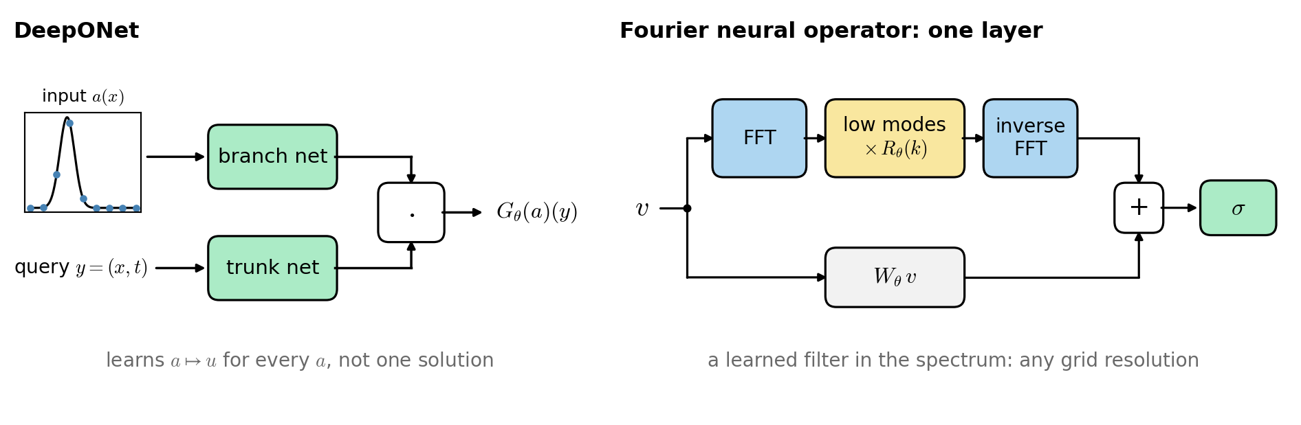
Neural Operators: Learn the Whole Solution Map

	Finite differences	PINN	Neural operator
Gives	one solution	one solution	a map: any input \(\mapsto\) its solution
Needs	the equation	the equation	many solver runs as training data
A new input costs	a full simulation	retraining	one forward pass, milliseconds
Autodiff is used for	gradients for inverse problems	input and weight derivatives	training; gradients w.r.t. the input for design
Watch out for	stability, dispersion	stalled training	inputs unlike the training data

\[ \frac{\partial^2 u}{\partial t^2} = \frac{\partial}{\partial x}\Big(\color{red}{a(x)}\frac{\partial u}{\partial x}\Big), \quad u(x,0)=u_0(x), \quad u_t(x,0)=v_0(x) \] cf. DeepONet, FNO

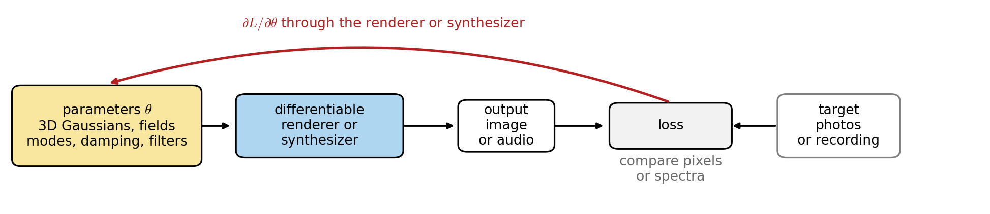
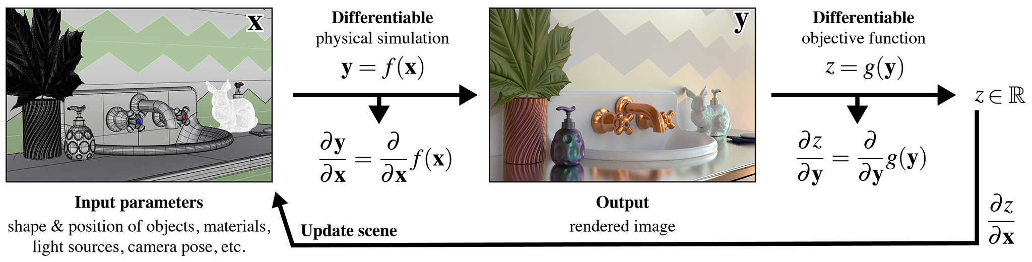
Differentiable Rendering and Sound

• 3D recon from photos (e.g. novel view synthesis)
  • Physically Based Rendering (PBR): Mitsuba 3, Cycles
  • ‘Simplified’ rendering + NN: NeRF, 3DGS, etc.
• The renderer plays the simulator by forward/backward
  • fit whatever parameters by differentiating through it.

Many other fields approach the similar way: Locomotion, Tactile sensing, Fluid simulation, etc.

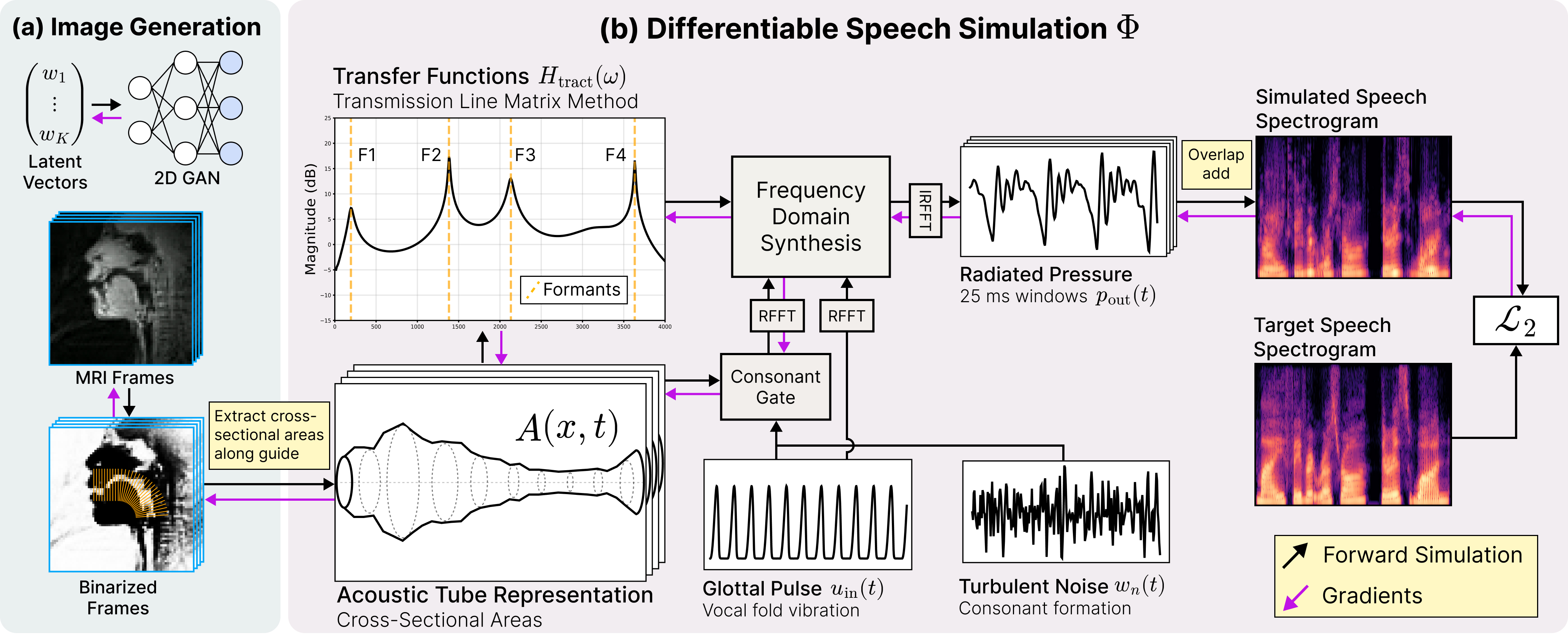
• Reproducing performance from recordings
  • Physical modellling synthesizers (for instrument modeling, acoustic scene reconstruction, …)
  • cf. DDSP shares the same approach but with abstract synthesis modules instead of physics-based ones.

Recap

Recap on Today’s ILO

• Describe what the computer does to get df/dx.
  • Run f(x) on tracked numbers: each operation writes a row of the tape. Seed \(\bar y=1\), read the tape backward, add \(\bar v\cdot\)(block derivative) to each parent. On a network: backpropagation.
• Explain physics-informed networks.
  • Differentiate a network with respect to its inputs, and the equation becomes the loss. The error moves from the derivative to the optimizer.
• List other autodiff-based methods.
  • Differentiable simulation, universal differential equations, solver in the loop, neural operators, differentiable rendering and sound: same engine, different unknowns.