Numerics and Error Analysis

Topics in Digital Heritage:
Numerical Methods for Digital Reconstruction

Jin Woo Lee

KAIST

Fall 2026

Topics in Digital Heritage

Digits

Digits

• Mesh: \(\big\{(0,0), (1,1), (2,0), (3,-1), (4,0)\big\}\)
  • \(y=\sin(\frac{\pi}{2}x)\) vs. \(y=x(x-2)(x-4)/3\) vs. …
  • Differences? Periodic? Aperiodic?

Today’s ILO

• Explain the mathematical concepts of linearity and non-linearity, convexity and non-convexity, and their implications in numerical methods.
• Implement basic error analysis technique to assess the numerical accuracy.
• Distinguish the types of errors in numerical computations and their impact on the accuracy of results.

Mathematics Review

Numbers and Sets

• Natural numbers \(\mathbb{N} = \{1, 2, 3, ...\}\)
• Integers \(\mathbb{Z} = \{..., -2, -1, 0, 1, 2, ...\}\)
• Rational numbers \(\mathbb{Q} = \left\{\frac{p}{q} : p \in \mathbb{Z}, q \in \mathbb{Z}\setminus \{0\}\right\}\)
• Real numbers \(\mathbb{R} = \{x : x \text{ is a limit of a convergent sequence of rational numbers}\}\)
  • Encompasses \(\mathbb{Q}\) as well as irrational numbers like \(\pi\), \(\sqrt{2}\), etc.
• Complex numbers \(\mathbb{C} = \{x + iy : x, y \in \mathbb{R}, i^2 = -1\}\)

Vector Spaces

A vector space \(V\) over \(\mathbb{R}\) is a set closed under addition and scalar multiplication, satisfying the following axioms:

Vector Space Axioms

1. Associativity: For all \(\mathbf{u}, \mathbf{v}, \mathbf{w} \in V\), \((\mathbf{u} + \mathbf{v}) + \mathbf{w} = \mathbf{u} + (\mathbf{v} + \mathbf{w})\).
2. Commutativity: For all \(\mathbf{u}, \mathbf{v} \in V\), \(\mathbf{u} + \mathbf{v} = \mathbf{v} + \mathbf{u}\).
3. Add. identity: There exists an element \(\mathbf{0} \in V\) such that \(\mathbf{v} + \mathbf{0} = \mathbf{v}\) for all \(\mathbf{v} \in V\).
4. Add. inverses: For every \(\mathbf{v} \in V\), there exists an element \(-\mathbf{v} \in V\) such that \(\mathbf{v} + (-\mathbf{v}) = \mathbf{0}\).
5. Distributivity: For all \(c,d \in \mathbb{R}\) and \(\mathbf{u}, \mathbf{v} \in V\), \(c(\mathbf{u} + \mathbf{v}) = c\mathbf{u} + c\mathbf{v}\) and \((c + d)\mathbf{v} = c\mathbf{v} + d\mathbf{v}\).
6. Mult. identity: For all \(\mathbf{v} \in V\), \(1\mathbf{v} = \mathbf{v}\), where \(1\) is the multiplicative identity in \(\mathbb{R}\).
7. Compatibility with field multiplication: For all \(c, d \in \mathbb{R}\) and \(\mathbf{v} \in V\), \((cd)\mathbf{v} = c(d\mathbf{v})\).

\(\mathbb{R}^2\) is a vector space

\(n\)-dimensional Euclidean Space \(\mathbb{R}^n\)

\(x\in\mathbb{R}\equiv\mathbb{R}^1\)

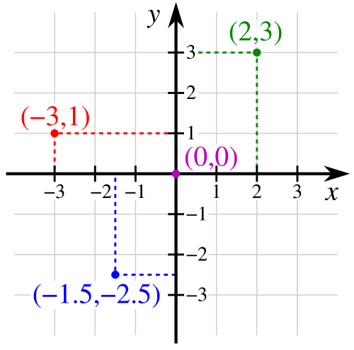
\((x,y)\in\mathbb{R}^2\)

\((x,y,z)\in\mathbb{R}^3\)

\((a_1, ..., a_n) \equiv \begin{bmatrix} a_1 \\ \vdots \\ a_n \end{bmatrix} \in \mathbb{R}^n\)

Linearity

Definition

A function \(f: \mathbb{R}^n \to \mathbb{R}^m\) is linear if it satisfies the following two properties for all \(\mathbf{u}, \mathbf{v} \in \mathbb{R}^n\) and all scalars \(c \in \mathbb{R}\):

1. Additivity: \(f(\mathbf{u} + \mathbf{v}) = f(\mathbf{u}) + f(\mathbf{v})\)
2. Homogeneity: \(f(c\mathbf{u}) = c f(\mathbf{u})\)

• \(y = 2x\) linear?
• \(y = 2x - 1\) linear?
• \(y = \sin(x)\) linear?

Linear System

\[\begin{split} 3x + 2y + 5z &= 0 \\ -4x + 9y - 3z &= -7 \\ 2x -3y -3z &= 1 \end{split}\]

\[ \begin{bmatrix} 3 & 2 & 5 \\ -4 & 9 & -3 \\ 2 & -3 & -3 \end{bmatrix} \begin{bmatrix} x \\ y \\ z \end{bmatrix} = \begin{bmatrix} 0 \\ -7 \\ 1 \end{bmatrix} \]

\[ \mathbf{A}\mathbf{x} = \mathbf{b} \]

If \(\exists \mathbf{A}^{-1}\), s.t. \(\mathbf{A}^{-1}\mathbf{A} = \mathbf{I}\), then \[\mathbf{x} = \mathbf{A}^{-1}\mathbf{b}.\]

Non-linearity

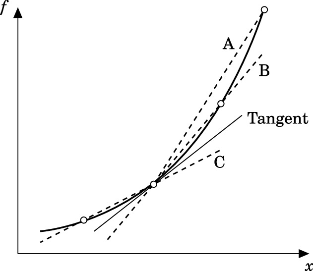
Local Linearity

\[f'(x_0) = \lim_{\Delta x\to 0}\frac{f(x_0 + \Delta x)-f(x_0)}{\Delta x}\]

\[ f'(x_0) = \frac{f(x_0 + \Delta x)-f(x_0)}{\Delta x} + \mathcal{O}(\Delta x^2) \]

\[ f(x_0 + \Delta x) = f(x_0) + f'(x_0){\Delta x} + \mathcal{O}(\Delta x^2) \]

\[ f(x_0 + \Delta x) = f(x_0) + f'(x_0){\Delta x} + f''(x_0)\frac{\Delta x^2}{2!} + \cdots + f^{(k)}(x_0)\frac{\Delta x^k}{k!} + \mathcal{O}(\Delta x^{k+1}) \]

Non-convexity

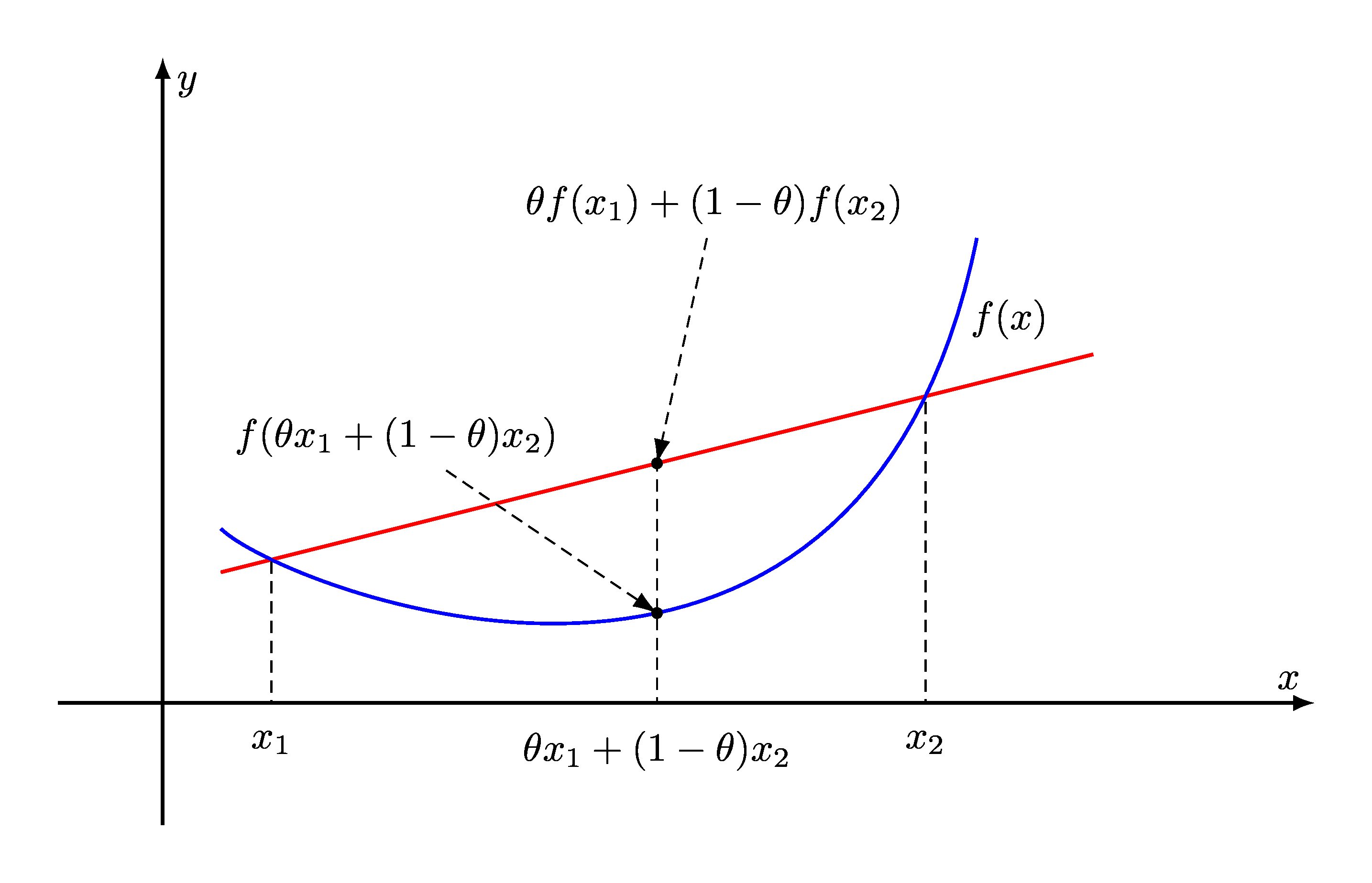
Convex Function

A function \(f: \mathbb{R}^n \to \mathbb{R}\) is convex if for all \(x_1, x_2 \in \mathbb{R}^n\) and \(\theta \in [0, 1]\): \[f(\theta x_1 + (1-\theta) x_2) \leq \theta f(x_1) + (1-\theta) f(x_2)\]

Non-convex Function

A function \(f: \mathbb{R}^n \to \mathbb{R}\) is non-convex if there exist \(x_1, y_2 \in \mathbb{R}^n\) and \(\theta \in [0, 1]\) such that: \[f(\theta x_1 + (1-\theta) x_2) > \theta f(x_1) + (1-\theta) f(x_2)\]

Optimization

(Equality) Constrained Optimization

\[\begin{aligned} \text{minimize } & f(\mathbf{x}) \\ \text{subject to } & g(\mathbf{x}) = 0 \end{aligned}\]

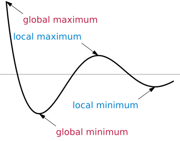
Numerics and Error Analysis

Storing Numbers with Fractional Parts

Binary Representation

• \(203 = 2^7 + 2^6 + 2^3 + 2^1 + 2^0 = 11001011_2\)
• \(203.625 = 2^7 + 2^6 + 2^3 + 2^1 + 2^0 + 2^{-1} + 2^{-3} = 11001011.101_2\)

Fractional and Irrational Numbers

• \(\frac{1}{3} = 0.33333333\cdots = 0.010101010101\cdots_2\)
• \(\pi = 11.00100100001\cdots_2\)

Storing Numbers with Fractional Parts

volatile double x = 1.0;
volatile double y = x / 3.0;
if (x == y * 3.0) {
    cout << "They are equal!" << endl;
} else {
    cout << "They are NOT equal." << endl;
    cout << "x: " << x << ", y: " << y << ", y*3: " << y * 3.0 << endl;
}

They are NOT equal.
x: 1, y: 0.333333, y*3: 0.999999

Note

Modern C++ compilers pre-compute constant expressions at compile time, applying “Round to Nearest” by default. So, the comparison x == y * 3.0 may yield true even if y is not exactly equal to 1/3, because the compiler optimizes the expression to if (1.0 == 1.0) at compile time.

Storing Numbers with Fractional Parts

volatile double x = 1.0;
volatile double y = x / 3.0;
if (std::abs(x - y * 3.0) < std::numeric_limits<double>::epsilon()) {
    cout << "They are equal!" << endl;
} else {
    cout << "They are NOT equal." << endl;
    cout << "x: " << x << ", y: " << y << ", y*3: " << y * 3.0 << endl;
}

They are equal!

Remark.

• Rarely if ever should the operator == and its equivalents be used on fractional values.
• Instead, some tolerance should be used to check if they are equal.

Fixed-Point, Floating-Point

Fixed-Point Representation

• Let’s say we have a fixed-point representation with 2 bits for the integer part and 2 bits for the fractional part.
  • \(\frac{1}{2} \cdot \frac{1}{2} = \frac{1}{4}\)    \(\Rightarrow\)    \(0.1_2 \cdot 0.1_2 = 0.01_2 \to 0.0_2\neq\frac{1}{4}\)

Floating-Point Representation

• Mass of an electron in kilograms: \(9.1093837015 \times 10^{-31}.\)
• The Avogadro constant: \(6.02214076 \times 10^{23} = 602,214,076,000,000,000,000,000.\)
• Represent numbers in \(a\times10^{e}\) where \(a\sim1\) and \(e\in\mathbb{Z}\).
  • The decimal point “floats” so that \(a\) is on a reasonable scale.

Understanding Errors

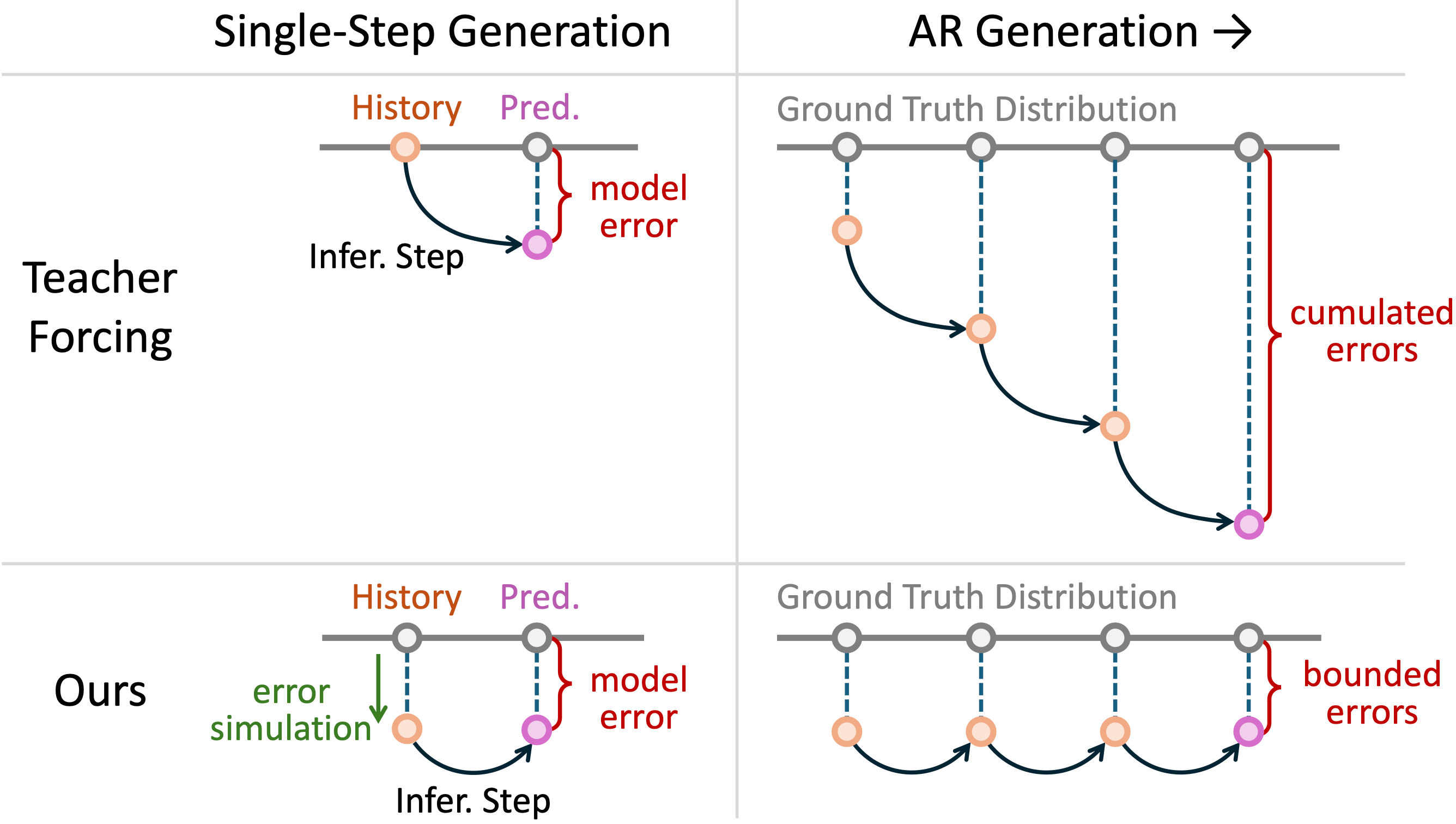
• Rounding (truncation) error
  • \(\pi = \color{red}{3.141592653589793}238462643383279502884197169399375\cdots\)

• Discretization error

• Cumulative error

• Modeling & Input error

Recap on Today’s ILO

Today’s ILO

• Explain the mathematical concepts of linearity and non-linearity, convexity and non-convexity, and their implications in numerical methods.
• Implement basic error analysis technique to assess the numerical accuracy.
• Distinguish the types of errors in numerical computations and their impact on the accuracy of results.