Linear Systems 2


Topics in Digital Heritage:
Numerical Methods for Digital Reconstruction

Jin Woo Lee

KAIST

Fall 2026

Recap

Solvability

The solvability of \(\mathbf{A}\mathbf{x} = \mathbf{b}\) must fall into one of three cases:

  1. The system may not admit any solutions, as in: \[ \begin{bmatrix} 1 & 0 \\ 1 & 0 \end{bmatrix} \begin{bmatrix} x \\ y \end{bmatrix} = \begin{bmatrix} -1 \\ 1 \end{bmatrix} \]

  2. The system may admit a single solution.

  3. The system may admit infinitely many solutions, e.g., \(0\mathbf{x} = \mathbf{0}\).

Non-square Matrices

  • No wide matrix system admits a unique solution.
  • For every tall matrix \(\mathbf{A}\), there exists a \(\mathbf{b}_0\) such that \(\mathbf{A}\mathbf{x} = \mathbf{b}_0\) is not solvable.

Least Squares (LS) Regression

We wish to solve the linear system \(\mathbf{A}\mathbf{x} = \mathbf{b}\), where \(\mathbf{A} \in \mathbb{R}^{m \times n}\) and \(\mathbf{b} \in \mathbb{R}^m\).

  • When we cannot solve \(\mathbf{A}\mathbf{x} = \mathbf{b}\) exactly, we can instead try to find an approximate solution \(\mathbf{x}\) satisfying \(\mathbf{A}\mathbf{x} \approx \mathbf{b}\).

This can be done by solving the least squares problem: \[\min_{\mathbf{x}} \|\mathbf{A}\mathbf{x} - \mathbf{b}\|^2_2\]

Tikhonov Reguliarization

When the system is ill-conditioned, we can add a regularization term to the least squares problem: \[\min_{\mathbf{x}} \|\mathbf{A}\mathbf{x} - \mathbf{b}\|^2_2 + \lambda \|\mathbf{x}\|^2_2\] where \(0 < \lambda \ll 1\). This second term is called the Tikhonov regularizer. This asks that among the minimizers of \(\|\mathbf{A}\mathbf{x} - \mathbf{b}\|_2^2\), we would prefer those with small norm \(\|\mathbf{x}\|_2\); as \(\lambda\) increases, we prioritize the norm of \(\mathbf{x}\) more.

  • The solution of the Tikhonov regularized problem is no longer exact.
  • When \(\lambda\) is small, the matrix \(\mathbf{A}^\top\mathbf{A} + \lambda \mathbf{I}\) is invertible but may be poorly conditioned. Increasing \(\lambda\) solves this at the cost of less accurate solutions.

Image Alignment

Given two images, we marked \(p\) pairs of points \(\mathbf{x}^{(k)},\mathbf{y}^{(k)}\in\mathbb{R}^2\) in each image. We want to find the best rotation and translation that aligns the two images.

Suppose that there exists some transformation matrix \(\mathbf{A}\in\mathbb{R}^{2\times 2}\) and translation vector \(\mathbf{b}\in\mathbb{R}^2\) such that: \[\mathbf{y}^{(k)} = \mathbf{A}\mathbf{x}^{(k)} + \mathbf{b}, \quad k=1, ..., p\]

Given a set of corresponding points \(\{\mathbf{x}^{(k)}, \mathbf{y}^{(k)}\}_{k=1}^p\), we can set up a linear system to solve for the unknowns in \(\mathbf{A}\) and \(\mathbf{b}\).

To do so, we solve the following minimization problem: \[\min_{\mathbf{A}, \mathbf{b}} \sum_{k=1}^p \|\mathbf{y}^{(k)} - (\mathbf{A}\mathbf{x}^{(k)} + \mathbf{b})\|^2_2\]

Deconvolution

  Blurry \(\mathbf{x}_0\quad\) Sharp \(\mathbf{x}\)

Given a blurry image \(\mathbf{x}_0\) and a known blur kernel \(\mathbf{h}\), we want to recover the original sharp image \(\mathbf{x}\). One strategy is deconvolution, which can be formulated as a linear system: \[\min_{\mathbf{x}} \|\mathbf{h} * \mathbf{x} - \mathbf{x}_0\|^2_2\] where \(*\) denotes convolution.

In this case, the unknown is \(\mathbf{x}\), where in many cases, multiple solutions may exist due to the ill-posed nature of the problem. This can be solved possibly with Tikhonov regularization.

Today’s ILO

  • Experiment with image alignment and deconvolution using least squares and Tikhonov regularization.
  • Implement the least squares solution for image alignment and deconvolution in Python.

Code Practices

Image Alignment

Image Alignment

Given two images, we marked \(p\) pairs of points \(\mathbf{x}^{(k)},\mathbf{y}^{(k)}\in\mathbb{R}^2\) in each image. We want to find the best rotation and translation that aligns the two images.

Suppose that there exists some transformation matrix \(\mathbf{A}\in\mathbb{R}^{2\times 2}\) and translation vector \(\mathbf{b}\in\mathbb{R}^2\) such that: \[\mathbf{y}^{(k)} = \mathbf{A}\mathbf{x}^{(k)} + \mathbf{b}, \quad k=1, ..., p\]

Given a set of corresponding points \(\{\mathbf{x}^{(k)}, \mathbf{y}^{(k)}\}_{k=1}^p\), we can set up a linear system to solve for the unknowns in \(\mathbf{A}\) and \(\mathbf{b}\).

To do so, we solve the following minimization problem: \[\min_{\mathbf{A}, \mathbf{b}} \sum_{k=1}^p \|\mathbf{y}^{(k)} - (\mathbf{A}\mathbf{x}^{(k)} + \mathbf{b})\|^2_2\]

Image Alignment

\[\min_{\mathbf{A}, \mathbf{b}} \sum_{k=1}^p \|\mathbf{y}^{(k)} - (\mathbf{A}\mathbf{x}^{(k)} + \mathbf{b})\|^2_2\] \[ \begin{split} f(\mathbf{A},\mathbf{b}) &\equiv \sum_{k} \|\mathbf{y}^{(k)} - (\mathbf{A}\mathbf{x}^{(k)} + \mathbf{b})\|^2_2 \\ &=\sum_k \left(\mathbf{x}^(k)^\top \mathbf{A}^\top \mathbf{A} \mathbf{x}^{(k)} + 2\mathbf{b}^\top \mathbf{A}\mathbf{x}^{(k)} + \mathbf{b}^\top \mathbf{b} - 2\mathbf{y}^{(k)\top}\mathbf{A}\mathbf{x}^{(k)} - 2\mathbf{y}^{(k)\top}\mathbf{b} + \mathbf{y}^{(k)\top}\mathbf{y}^{(k)}\right) \end{split}\]

\[\begin{split} 0 = \frac{\partial}{\partial \mathbf{A}} f(\mathbf{A},\mathbf{b}) &= \sum_{k=1}^p \left(2\mathbf{A}\mathbf{x}^{(k)}\mathbf{x}^{(k)\top} + 2\mathbf{b}\mathbf{x}^{(k)\top} - 2\mathbf{y}^{(k)}\mathbf{x}^{(k)\top}\right) \\ &\Rightarrow \mathbf{A}\mathbf{x}_\mathrm{sum}\mathbf{x}_\mathrm{sum}^\top + \mathbf{b}\mathbf{x}_\mathrm{sum}^\top = \mathbf{y}_\mathrm{sum}\mathbf{x}_\mathrm{sum}^\top \\ &\Rightarrow \boxed{\mathbf{A}\mathbf{X} + \mathbf{b}\mathbf{x}_\mathrm{sum}^\top = \mathbf{C}} \\ 0 = \frac{\partial}{\partial \mathbf{b}} f(\mathbf{A},\mathbf{b}) &= \sum_{k=1}^p \left(2\mathbf{A}\mathbf{x}^{(k)} + 2\mathbf{b} - 2\mathbf{y}^{(k)}\right) \\ &\Rightarrow \boxed{\mathbf{A}\mathbf{x}_\mathrm{sum} + p\mathbf{b} = \mathbf{y}_\mathrm{sum}} \end{split}\]

Image Alignment

Stack the source/target points as rows of a design matrix, with an extra column of ones for the intercept \(\mathbf{b}\)

\[ \mathbf{Z} = \begin{bmatrix} \mathbf{x}^{(1)\top} & 1 \\ \vdots & \vdots \\ \mathbf{x}^{(p)\top} & 1 \end{bmatrix} \in \mathbb{R}^{p \times 3}, \qquad \mathbf{Y} = \begin{bmatrix} \mathbf{y}^{(1)\top} \\ \vdots \\ \mathbf{y}^{(p)\top} \end{bmatrix} \in \mathbb{R}^{p \times 2} \]

Then

\[ \mathbf{Z}^\top \mathbf{Z} = \begin{bmatrix} \mathbf{x}_\mathrm{sum}\mathbf{x}_\mathrm{sum}^\top & \mathbf{x}_\mathrm{sum} \\ \mathbf{x}_\mathrm{sum}^\top & p \end{bmatrix}, \qquad \mathbf{Z}^\top \mathbf{Y} = \begin{bmatrix} (\mathbf{y}_\mathrm{sum}\mathbf{x}_\mathrm{sum}^\top)^\top \\ \mathbf{y}_\mathrm{sum}^\top \end{bmatrix} \]

so that, writing \(\mathbf{W} = \begin{bmatrix} \mathbf{A}^\top \\ \mathbf{b}^\top \end{bmatrix} \in \mathbb{R}^{3\times 2}\), the normal equation

\[\boxed{\mathbf{Z}^\top \mathbf{Z}\, \mathbf{W} = \mathbf{Z}^\top \mathbf{Y}}\]

is block-row-wise just the transpose of \(\mathbf{A}\mathbf{X} + \mathbf{b}\mathbf{x}_\mathrm{sum}^\top = \mathbf{C}\) and \(\mathbf{A}\mathbf{x}_\mathrm{sum} + p\mathbf{b} = \mathbf{y}_\mathrm{sum}\).

Image Alignment

Practice!

Go to the Colab Notebook

Deconvolution

Deconvolution

Given a blurry image \(\mathbf{x}_0\) and a known blur kernel \(\mathbf{h}\), we want to recover the original sharp image \(\mathbf{x}\). One strategy is deconvolution, which can be formulated as a linear system: \[\min_{\mathbf{x}} \|\mathbf{h} * \mathbf{x} - \mathbf{x}_0\|^2_2\] where \(*\) denotes convolution.

In this case, the unknown is \(\mathbf{x}\), where in many cases, multiple solutions may exist due to the ill-posed nature of the problem. This can be solved possibly with Tikhonov regularization.

Deconvolution

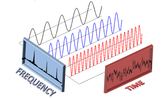
Convolution Theorem

Convolution \[ (f * g)(t) = \int_{-\infty}^{\infty} f(\tau) g(t - \tau) d\tau \]

Fourier Transform \[ \mathcal{F}\{ x(t) \} = X(f) = \int_{-\infty}^{\infty} x(t) e^{-j 2 \pi f t} dt \]

\[\begin{aligned} \mathcal{F}\{ f * g \} &= \int_{-\infty}^{\infty} (f * g)(t) e^{-j 2 \pi f t} dt \\ &= \int_{-\infty}^{\infty} \left( \int_{-\infty}^{\infty} f(\tau) g(t - \tau) d\tau \right) e^{-j 2 \pi f t} dt \\ &= \int_{-\infty}^{\infty} f(\tau) \left( \int_{-\infty}^{\infty} g(t - \tau) e^{-j 2 \pi f t} dt \right) d\tau \\ &= \int_{-\infty}^{\infty} f(\tau) \left( \int_{-\infty}^{\infty} g(u) e^{-j 2 \pi f (u + \tau)} du \right) d\tau \\ &\qquad\qquad\qquad\qquad\qquad (u = t - \tau;\ dt=du) \\ &= \int_{-\infty}^{\infty} f(\tau) e^{-j 2 \pi f \tau} \left( \int_{-\infty}^{\infty} g(u) e^{-j 2 \pi f u} du \right) d\tau \\ &= \left( \int_{-\infty}^{\infty} f(\tau) e^{-j 2 \pi f \tau} d\tau \right) \left( \int_{-\infty}^{\infty} g(u) e^{-j 2 \pi f u} du \right) \\ &= \mathcal{F}\{f\} \cdot \mathcal{F}\{g\} \end{aligned}\]

Deconvolution (complex)

The objective function \[\min_{\mathbf{x}} \|\mathbf{h} * \mathbf{x} - \mathbf{x}_0\|^2_2 + \lambda \|\mathbf{x}\|_2^2\] can be rewritten in the frequency domain using the convolution theorem: \[ \min_{\mathbf{x}} \|\mathbf{H} \cdot \mathbf{X} - \mathbf{X}_0\|^2_2 + \lambda \|\mathbf{X}\|_2^2\] where \(\mathbf{H} = \mathcal{F}\{\mathbf{h}\}\) and \(\mathbf{X} = \mathcal{F}\{\mathbf{x}\}\). Taking derivatives and setting them to zero, we get the normal equation \(\mathbf{H}^* \cdot (\mathbf{H} \cdot \mathbf{X} - \mathbf{X}_0) + \lambda \mathbf{X} = 0\), or \[ \boxed{\mathbf{X} = \frac{\mathbf{H}^* \cdot \mathbf{X}_0}{|\mathbf{H}|^2 + \lambda}} \]

Deconvolution

Practice!

Go to the Colab Notebook