Iterative Linear Solvers
Topics in Digital Heritage:
Numerical Methods for Digital Reconstruction
Fall 2026
From Last Class: Newton’s Method
Recall Newton’s method for root-finding, \[x_{k+1} = x_k - \frac{f(x_k)}{f'(x_k)}\].
Its multivariate generalization for minimizing \(f(\mathbf{x})\) takes a step \[ \mathbf{x}_{k+1} = \mathbf{x}_k - \left[\nabla^2 f(\mathbf{x}_k)\right]^{-1} \nabla f(\mathbf{x}_k), \] i.e. it solves a linear system every single iteration: \[ \underbrace{\nabla^2 f(\mathbf{x}_k)}_{\mathbf{A}} \, \underbrace{(\mathbf{x}_{k+1} - \mathbf{x}_k)}_{\mathbf{v}} = -\underbrace{\nabla f(\mathbf{x}_k)}_{\mathbf{b}}. \]
Solving \(\mathbf{A}\mathbf{v} = \mathbf{b}\) can be done exactly, yet costing \(O(n^3)\).
- Gaussian elimination, LU, Cholesky, … \(\to\) slow when \(n\) is large.

Why Look for Something Else?
- Many \(\mathbf{A}\)’s that show up in practice (discretized images, meshes, grids, graphs) are large and sparse: mostly zeros.
- Gaussian elimination tends to fill in those zeros as it proceeds, so we can lose the sparsity that made the problem tractable to store in the first place.
- We often only need \(\mathbf{A}\) applied to a vector \(\mathbf{x}\), (i.e. \(\mathbf{A}\mathbf{x}\)), not \(\mathbf{A}\) itself in explicit matrix form.
- Sometimes an approximate \(\mathbf{x}\) found in a handful of cheap steps is good enough, e.g. inside an outer loop like Newton’s method above.
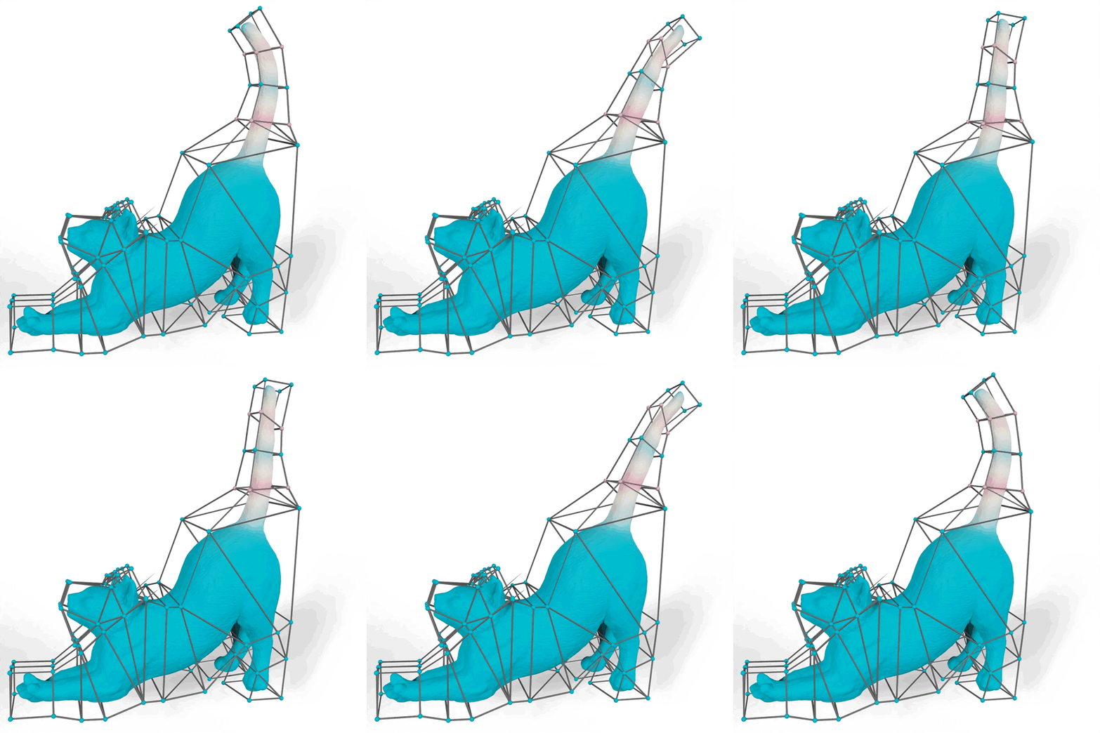
- 3D meshes with \(m>10^{4}\) vertices (\(n=3m\) number of unknowns) yield \(3m\times 3m\) sparse matrices \(\mathbf{A}\).
- Directly solving \(\mathbf{A}\mathbf{x}=\mathbf{b}\) with cost of \(O((3m)^3)\) is prohibitive in such cases.
- Saving \(\mathbf{A}\) in memory is wasteful, since we only need \(\mathbf{A}\mathbf{x}\) for some vector \(\mathbf{x}\).
Today: solve \(\mathbf{A}\mathbf{x}=\mathbf{b}\) by turning it into a minimization problem and attacking it iteratively, with no factorization required.
Visualizing the Quadratic Energy
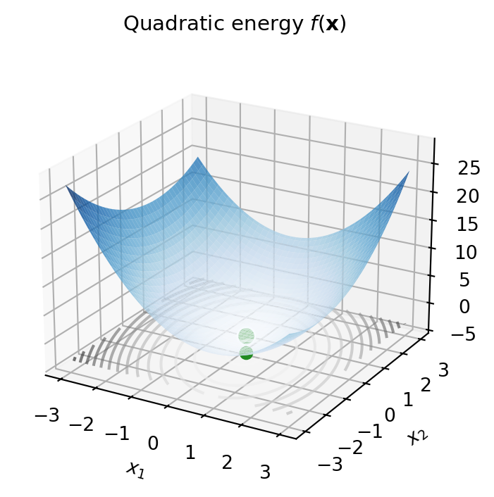
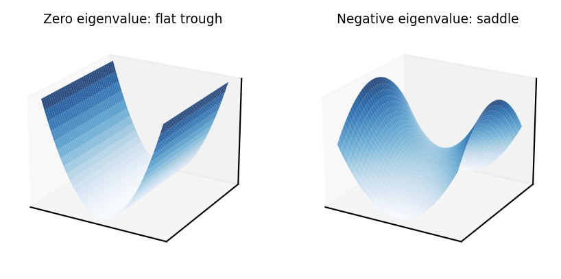
For \(n=2\), \(f(\mathbf{x})\) is a surface over the plane: a paraboloid bowl exactly when \(\mathbf{A}\) is SPD.
Why a bowl?
\[ f(\mathbf{x}) = f(\mathbf{x}^*) + \frac{1}{2}(\mathbf{x}-\mathbf{x}^*)^\top \mathbf{A} (\mathbf{x}-\mathbf{x}^*), \qquad \mathbf{x}^* = \mathbf{A}^{-1}\mathbf{b} \] Since \(\mathbf{A}\) is PD, the second term is strictly positive whenever \(\mathbf{x}\neq\mathbf{x}^*\), so \(f\) increases in every direction away from \(\mathbf{x}^*\).
Details
\[\begin{aligned} f(\mathbf{x}) &= \frac{1}{2}\mathbf{x}^\top\mathbf{A}\mathbf{x} - \mathbf{b}^\top\mathbf{x} + c \\ &= \frac{1}{2}\mathbf{x}^\top\mathbf{A}\mathbf{x} - (\mathbf{A}\mathbf{x}^*)^\top\mathbf{x} + c \\ &= \frac{1}{2}\mathbf{x}^\top\mathbf{A}\mathbf{x} - (\mathbf{x}^*)^\top\mathbf{A}\mathbf{x} + c \\ &= \frac{1}{2}\mathbf{x}^\top\mathbf{A}\mathbf{x} - (\mathbf{x}^*)^\top\mathbf{A}\mathbf{x} + \frac{1}{2}(\mathbf{x}^*)^\top\mathbf{A}\mathbf{x}^* - \frac{1}{2}(\mathbf{x}^*)^\top\mathbf{A}\mathbf{x}^* + c \\ &= \frac{1}{2}(\mathbf{x}-\mathbf{x}^*)^\top \mathbf{A} (\mathbf{x}-\mathbf{x}^*) + f(\mathbf{x}^*). \end{aligned}\]
\[\begin{aligned} \nabla f(\mathbf{x}^*) &= \mathbf{A}\mathbf{x}^* - \mathbf{b} = \mathbf{0} \\ \implies \mathbf{b} &= \mathbf{A}\mathbf{x}^*. \\ f(\mathbf{x}^*) &= \frac{1}{2}(\mathbf{x}^*)^\top\mathbf{A}\mathbf{x}^* - (\mathbf{x}^*)^\top\mathbf{b} + c \\ &= \frac{1}{2}(\mathbf{x}^*)^\top\mathbf{A}\mathbf{x}^* - (\mathbf{x}^*)^\top\mathbf{A}\mathbf{x}^* + c \\ &= -\frac{1}{2}(\mathbf{x}^*)^\top\mathbf{A}\mathbf{x}^* + c. \end{aligned}\]
- The lowest point of this bowl is exactly \(\mathbf{x}^*\)
- Minimizing \(f\) \(\iff\) solving the linear system
cf. A negative eigenvalue would give a saddle; a zero eigenvalue gives a flat trough.
Level Sets and the Shape of the Bowl
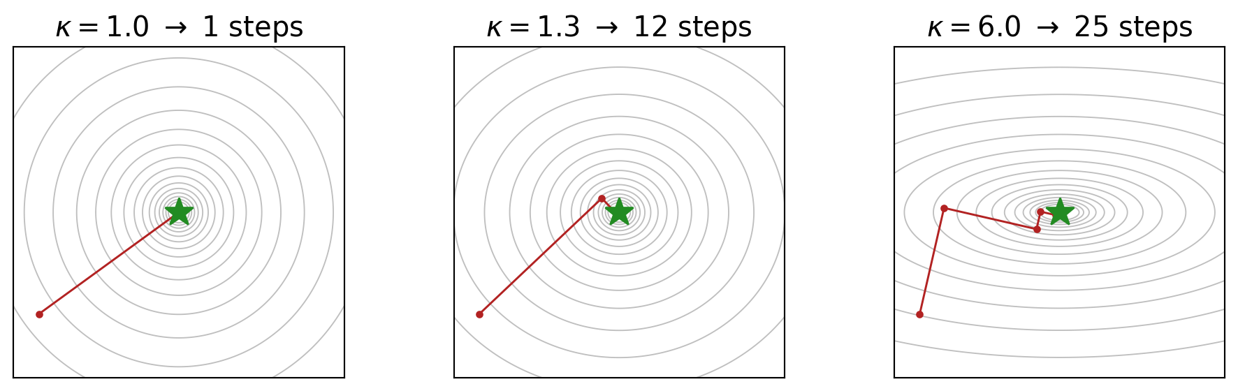
Looking at the bowl from directly above, its level sets (contours of equal \(f\) value) are ellipses. Their axes point along the eigenvectors of \(\mathbf{A}\), with lengths set by the eigenvalues:
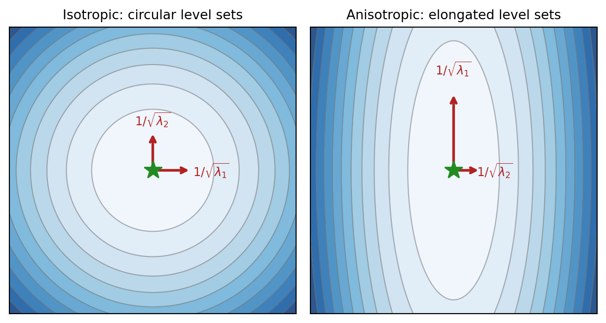
- Round bowl:
- eigenvalues close together
- easy to descend directly.
- Stretched bowl:
- eigenvalues far apart, i.e. large \(\text{cond}(\mathbf{A})\)
- easy to overshoot across the short axis
- slow to cross along the long one \(\to\) zig-zagging.
Watching Gradient Descent Descend
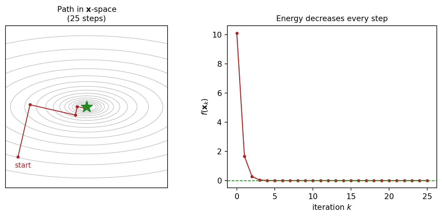
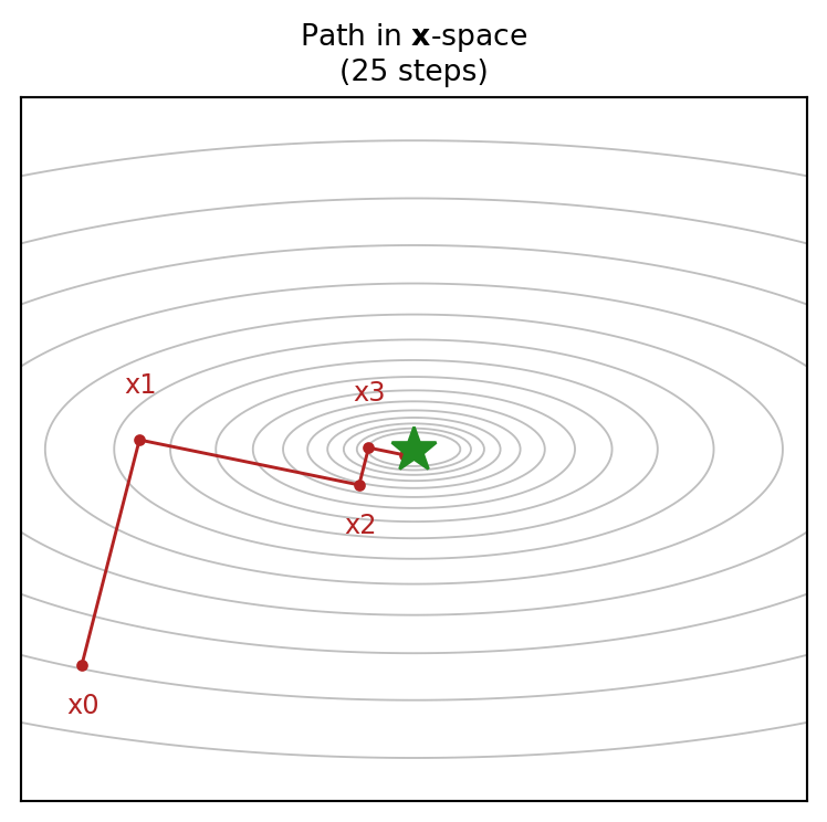
- Each step turns exactly 90 degrees from the last (a property of exact line search on a quadratic).
- \(f(\mathbf{x}_k)\) drops monotonically, but progress stalls once the path lines up with the bowl’s long axis.
Gradient Descent Algorithm
def gradient_descent(matvec, b, x0, tol=1e-8, max_iter=1000):
    x = x0.copy()
    r = b - matvec(x)                    # residual = search direction
    for k in range(max_iter):
        if norm(r) < tol * norm(b):      # stopping condition
            return x
        alpha = (r @ r) / (r @ matvec(r))  # closed-form step size
        x = x + alpha * r
        r = b - matvec(x)
    return x
\[\alpha_k = \frac{\mathbf{r}_k^\top \mathbf{r}_k}{\mathbf{r}_k^\top \mathbf{A} \mathbf{r}_k}\qquad \mathbf{x}_k = \mathbf{x}_{k-1} + \alpha_k \mathbf{r}_k\]
Notice: \(\mathbf{A}\) is only ever used through matvec(x) \(= \mathbf{A}\mathbf{x}\), never formed or factored explicitly. This is what lets it scale to huge sparse systems.
Convergence: It’s All About Conditioning
Linear convergence rate
Gradient descent converges unconditionally, but the rate depends only on the condition number \(\kappa = \text{cond}(\mathbf{A})\): \[ \frac{f(\mathbf{x}_k)-f(\mathbf{x}^*)}{f(\mathbf{x}_{k-1})-f(\mathbf{x}^*)} \;\le\; 1-\frac{1}{\kappa}. \]
Intuition: a well-conditioned \(\mathbf{A}\) has a round bowl, so steepest descent points straight at the minimum. A poorly-conditioned \(\mathbf{A}\) has a narrow valley, so steepest descent zig-zags across it, making painfully slow progress along the valley floor.
Why Gradient Descent Wastes Work
Zig-zagging is a symptom of a deeper issue: gradient descent may search along a direction it has already (partially) explored, undoing part of its own progress.
Idea
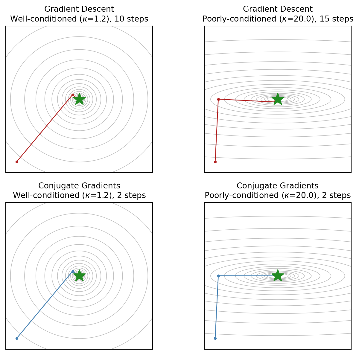
What if we picked \(n\) search directions \(\mathbf{v}_1,\dots,\mathbf{v}_n\) that never “interfere” with each other, and did one exact line search along each? Then we’d reach \(\mathbf{x}^*\) in at most \(n\) steps, no revisiting required.
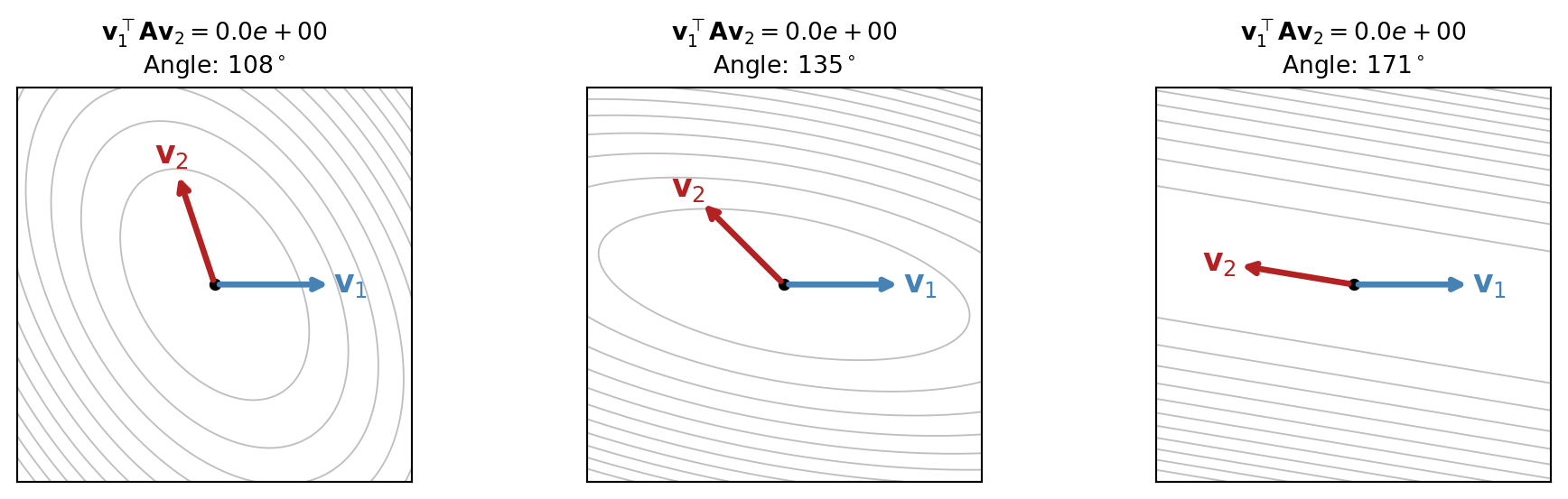
\(\mathbf{v}_1,\mathbf{v}_2\) are far from geometrically perpendicular, yet \(\mathbf{v}_1^\top\mathbf{A}\mathbf{v}_2=0\): they are “orthogonal” with respect to \(\mathbf{A}\)’s own geometry, exactly the ellipse’s own axes-like directions.
GD vs. CG
Scaling to Larger Systems
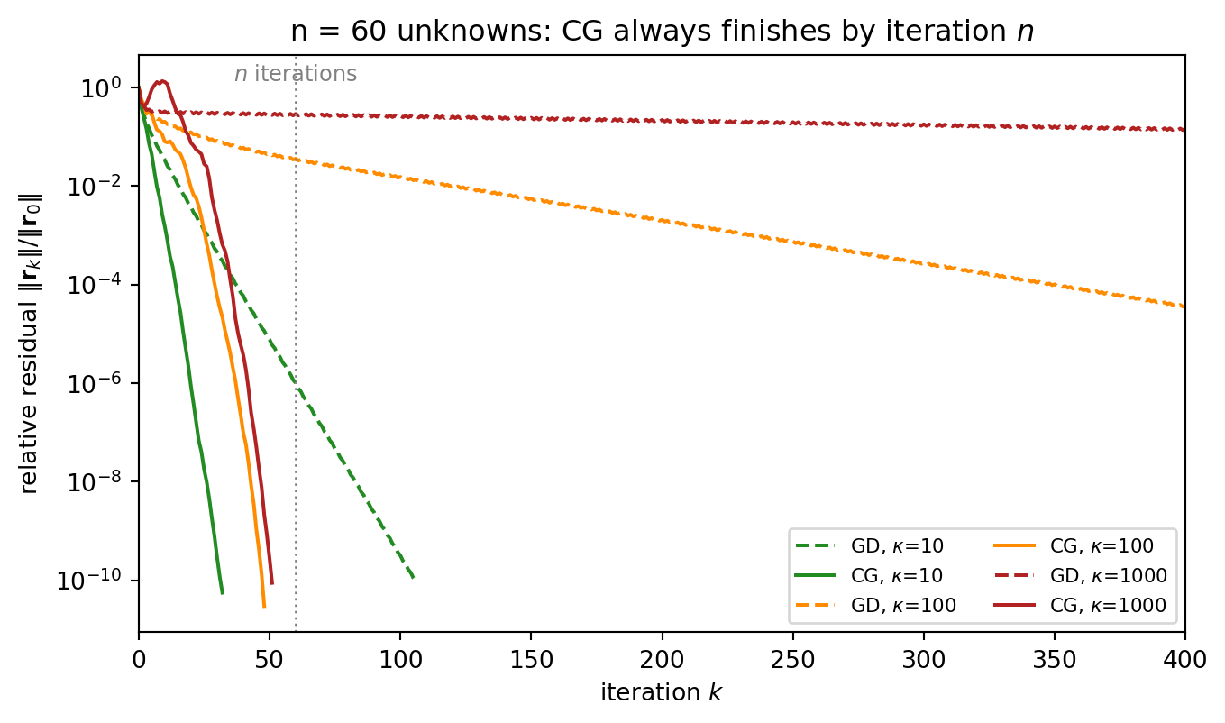
Dashed (GD) degrades sharply as \(\kappa\) grows; solid (CG) always converges by iteration \(n=60\), regardless of \(\kappa\), exactly as guaranteed.
Sneak Peek: A Discrete Poisson Equation
Poisson equation \(\nabla^2 u = f\) on a 60x60 grid, with 4 point sources/sinks. We frame this in a matrix-vector form \(\mathbf{A}\mathbf{u} = \mathbf{f}\) with \(\mathbf{A}\) never built explicitly; and apply CG to solve it.
Code
def laplacian_matvec(u_flat, N):
    u = u_flat.reshape(N, N)
    lap = -4.0 * u
    lap[1:, :] += u[:-1, :]; lap[:-1, :] += u[1:, :]
    lap[:, 1:] += u[:, :-1]; lap[:, :-1] += u[:, 1:]
    return -lap.ravel()          # matrix is never built; this is just a 5-point stencil

N = 60
b_grid = np.zeros((N, N))
b_grid[N // 4, N // 4] = 6.0;         b_grid[3 * N // 4, 3 * N // 4] = -6.0
b_grid[N // 4, 3 * N // 4] = 4.0;     b_grid[3 * N // 4, N // 4] = -4.0
b_flat = b_grid.ravel()
matvec = lambda u: laplacian_matvec(u, N)
x_sol = conjugate_gradient(matvec, b_flat, np.zeros(N * N), tol=1e-8, max_iter=N * N)
res = [np.linalg.norm(b_flat - matvec(x)) for x in x_sol[::max(1, len(x_sol)//200)]]

fig, axes = plt.subplots(1, 2, figsize=(8, 3))
im = axes[0].imshow(x_sol[-1].reshape(N, N), cmap="RdBu_r",
                     vmin=-np.abs(x_sol[-1]).max(), vmax=np.abs(x_sol[-1]).max())
axes[0].set_title("Solved field $u$\n(4 point sources/sinks)"); axes[0].axis("off")
plt.colorbar(im, ax=axes[0], fraction=0.046)
axes[1].semilogy(np.array(res) / res[0], color="steelblue")
axes[1].set_xlabel("CG iteration (subsampled)"); axes[1].set_ylabel("relative residual")
axes[1].set_title(f"Same CG code, n={N*N} unknowns\nno matrix ever built")
plt.tight_layout()
plt.show()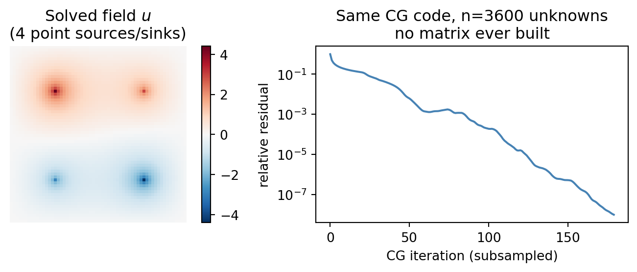
This is literally later-this-semester’s territory (Poisson/heat-diffusion equations), solved today with the same 10-line CG loop, applied through a stencil instead of a matrix.