Specialized Optimization Methods


Topics in Digital Heritage:
Numerical Methods for Digital Reconstruction

Jin Woo Lee

KAIST

Fall 2026

Recap

From the Last Two Classes: Two Generic Workhorses

Newton’s method (Class 5)

Minimizes any smooth \(f(\mathbf{x})\) by repeatedly solving \[\nabla^2 f(\mathbf{x}_k)\, \mathbf{d}_k = -\nabla f(\mathbf{x}_k)\] and stepping to \(\mathbf{x}_{k+1}=\mathbf{x}_k+\mathbf{d}_k\).

  • Needs the full Hessian every step.
  • Makes no assumption about the shape of \(f\).

Conjugate gradients (Class 6)

Minimizes exactly the quadratic energy \[f(\mathbf{x})=\tfrac12\mathbf{x}^\top\mathbf{A}\mathbf{x}-\mathbf{b}^\top\mathbf{x}\] matrix-free, guaranteed in \(\le n\) steps.

  • Only works when \(f\) is exactly this quadratic form.

Why Look for Something Else?

Real objectives are rarely “any smooth \(f\)” or “exactly quadratic”. They often have exploitable structure:

  • The objective is a sum of squared residuals (curve fitting, alignment).
  • The variables split naturally into blocks (rotations vs. positions, cluster labels vs. centers).
  • The landscape has many local minima that trap Newton-type methods.

Today: turn each kind of structure into an algorithm that is faster, simpler, or more robust than calling generic Newton or CG.

Today’s ILO

  • Explain how Gauss-Newton specializes Newton’s method for sum-of-squares objectives by linearizing residuals instead of building a Hessian, and implement it, along with its damped variant Levenberg-Marquardt.
  • Explain the coordinate descent / alternating optimization strategy, and implement it end-to-end on a concrete example (k-means clustering).
  • Recognize how global-search heuristics (graduated optimization, randomized search) extend these ideas further.
  • Preview where these specialized solvers resurface: automatic differentiation, ODE/PDE solvers, and fitting physical models later this semester.

Nonlinear Least Squares

From Linear to Nonlinear Regression

Recall linear least squares from Linear Systems 2: minimize \(\|\mathbf{A}\mathbf{x}-\mathbf{b}\|_2^2\).

Nonlinear least squares

Given functions \(f_1(\mathbf{x}),\dots,f_k(\mathbf{x})\) we want \(\approx \mathbf{0}\), minimize \[ E(\mathbf{x}) \equiv \frac{1}{2}\sum_i [f_i(\mathbf{x})]^2. \]

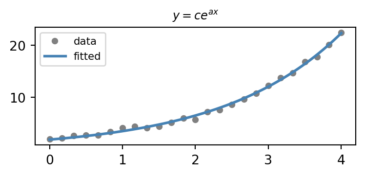
Example: fit \(y=ce^{ax}\) to data \((x_1,y_1),\dots,(x_k,y_k)\):

  • Take \(f_i(a,c) \equiv y_i - ce^{ax_i}\).
  • \(f_i\) is now nonlinear in the unknowns \(\mathbf{x}=(a,c)\)
  • There is no normal-equation shortcut.

Linearize and Repeat: The Gauss-Newton Idea

Linearize each \(f_i\) around the current estimate \(\mathbf{x}_t\) (Taylor expansion): \[ f_i(\color{red}{\mathbf{x}}) \approx f_i(\mathbf{x}_t) + \nabla f_i(\mathbf{x}_t)\cdot(\color{red}{\mathbf{x}}-\mathbf{x}_t). \]

Stacking the \(f_i\)’s into \(F(\mathbf{x})\) with Jacobian \(DF\), this turns \(E(\mathbf{x})\) into a linear least-squares problem in \(\color{blue}{\delta\mathbf{x}}=\color{red}{\mathbf{x}}-\mathbf{x}_t\): \[ \min_{\color{blue}{\delta\mathbf{x}}} \ \tfrac12\|F(\mathbf{x}_t) + DF(\mathbf{x}_t)\,\color{blue}{\delta\mathbf{x}}\|_2^2\]

which has the closed-form solution (derived shortly)

\[\boxed{\mathbf{x}_{t+1} = \mathbf{x}_t - \big(DF(\mathbf{x}_t)^\top DF(\mathbf{x}_t)\big)^{-1} DF(\mathbf{x}_t)^\top F(\mathbf{x}_t)} \]

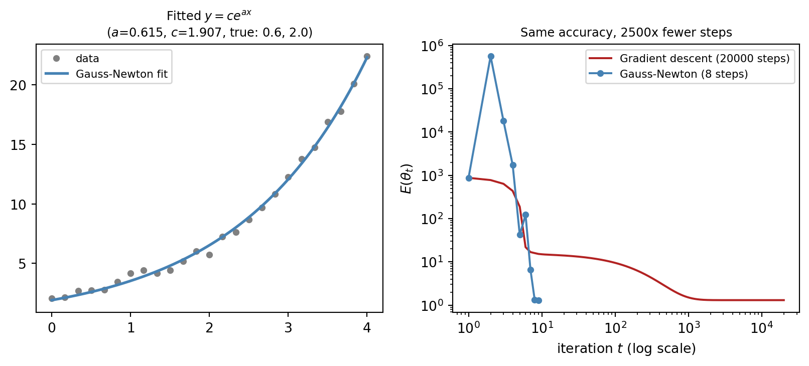
Iterating this update is Gauss-Newton. It only ever needs the first-order Jacobian \(DF\), never a Hessian, yet converges as fast as Newton’s method once close to the answer.

Framing as a Linear Least Squares Problem

Stack the Tangents, Then Substitute

Stack residuals into \(F(\mathbf{x})\in\mathbb{R}^k\) and gradients (as rows) into the Jacobian \(DF(\mathbf{x})\in\mathbb{R}^{k\times n}\). All \(k\) tangents then become one vector equation, with row \(i\) being exactly the tangent of \(f_i\): \[ \underbrace{\begin{bmatrix} f_1(\mathbf{x})\\ \vdots\\ f_k(\mathbf{x})\end{bmatrix}}_{F(\mathbf{x})} \approx \begin{bmatrix} f_1(\mathbf{x}_t) + \nabla f_1(\mathbf{x}_t)^\top\delta\mathbf{x}\\ \vdots\\ f_k(\mathbf{x}_t) + \nabla f_k(\mathbf{x}_t)^\top\delta\mathbf{x}\end{bmatrix} = \underbrace{\begin{bmatrix} f_1(\mathbf{x}_t)\\ \vdots\\ f_k(\mathbf{x}_t)\end{bmatrix}}_{F(\mathbf{x}_t)} + \underbrace{\begin{bmatrix} \nabla f_1(\mathbf{x}_t)^\top\\ \vdots\\ \nabla f_k(\mathbf{x}_t)^\top\end{bmatrix}}_{DF(\mathbf{x}_t)}\delta\mathbf{x}. \]

Since \(E(\mathbf{x}) = \tfrac12\sum_i f_i(\mathbf{x})^2 = \tfrac12\|F(\mathbf{x})\|_2^2\), just substitute the approximation: \[ E(\mathbf{x}_t+\delta\mathbf{x}) \;\approx\; \tfrac12\big\|F(\mathbf{x}_t) + DF(\mathbf{x}_t)\,\delta\mathbf{x}\big\|_2^2. \]

  • Inside the norm: (fixed vector) + (fixed matrix) \(\times\,\delta\mathbf{x}\)
  • This is a linear least-squares problem in \(\delta\mathbf{x}\).

Framing as a Linear Least Squares Problem

Squared Tangents Make a Parabola
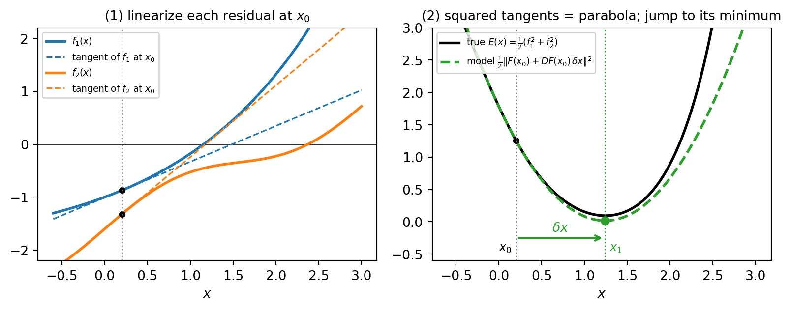
  • A sum of squared lines is always a quadratic in \(\delta\mathbf{x}\), so its minimizer has a closed form (will see next slide).
  • We repeat this linearization at the new point \(\mathbf{x}_1\), and so on, until convergence.

Finding the Minimizer in Closed Form

Rename \(A \equiv DF(\mathbf{x}_t)\) and \(\mathbf{b} \equiv -F(\mathbf{x}_t)\). The problem is exactly linear regression: \[ \min_{\delta\mathbf{x}}\ \tfrac12\|F(\mathbf{x}_t) + DF(\mathbf{x}_t)\,\delta\mathbf{x}\|_2^2 \;=\; \min_{\delta\mathbf{x}}\ \tfrac12\|A\,\delta\mathbf{x} - \mathbf{b}\|_2^2 . \]

Set the gradient to zero, which gives the normal equations: \[\begin{align*} \nabla_{\delta\mathbf{x}}\,\tfrac12\|A\,\delta\mathbf{x} - \mathbf{b}\|_2^2 = A^\top(A\,\delta\mathbf{x} - \mathbf{b}) = \mathbf{0} &\implies A^\top A\,\delta\mathbf{x} = A^\top\mathbf{b} \\ &\implies \delta\mathbf{x} = (A^\top A)^{-1}A^\top\mathbf{b}. \end{align*}\]

Rename back (\(A = DF(\mathbf{x}_t)\), \(\mathbf{b} = -F(\mathbf{x}_t)\)) and take the step \(\mathbf{x}_{t+1} = \mathbf{x}_t + \delta\mathbf{x}\): \[ \boxed{\mathbf{x}_{t+1} = \mathbf{x}_t - \big(DF(\mathbf{x}_t)^\top DF(\mathbf{x}_t)\big)^{-1} DF(\mathbf{x}_t)^\top F(\mathbf{x}_t)} \] This needs \(DF(\mathbf{x}_t)\) to have full column rank. We will see an alternative later in case this fails (Levenberg-Marquardt).

The Gauss-Newton Algorithm


def gauss_newton(F, DF, x0, max_iter=20):
    x = x0.copy()
    for t in range(max_iter):
        J = DF(x)              # Jacobian, shape (k, n)
        r = F(x)               # residual vector, shape (k,)
        delta, *_ = np.linalg.lstsq(J, -r, rcond=None) # solves: J delta = -r
        x = x + delta
    return x


  • Solves \(DF\,\delta\mathbf{x}=-F\) each step. This can be approached using:
    • Normal equations \(DF^\top DF\,\delta\mathbf{x} = -DF^\top F\), or
    • Conjugate gradients (matrix-free), etc.
    • We implement using np.linalg.lstsq (automatically chooses the best method).

Demo: Gauss-Newton Converges Fast

Back to the Nonlinear Regression Example

Show code
import numpy as np
import matplotlib.pyplot as plt

rng = np.random.default_rng(0)
a_true, c_true = 0.6, 2.0
x_data = np.linspace(0, 4, 25)
y_data = c_true * np.exp(a_true * x_data) + rng.normal(scale=0.4, size=x_data.size)

def residual(theta):
    a, c = theta
    return y_data - c * np.exp(a * x_data)

def jacobian(theta):
    a, c = theta
    e = np.exp(a * x_data)
    J = np.zeros((x_data.size, 2))
    J[:, 0] = -c * x_data * e
    J[:, 1] = -e
    return J

def loss(theta):
    r = residual(theta)
    return 0.5 * r @ r

def gradient_descent(theta0, lr, max_iter):
    theta = np.array(theta0, dtype=float)
    hist = [theta.copy()]
    for _ in range(max_iter):
        theta = theta - lr * (jacobian(theta).T @ residual(theta))
        hist.append(theta.copy())
    return np.array(hist)

def gauss_newton(theta0, max_iter):
    theta = np.array(theta0, dtype=float)
    hist = [theta.copy()]
    for _ in range(max_iter):
        J, r = jacobian(theta), residual(theta)
        delta, *_ = np.linalg.lstsq(J, -r, rcond=None)
        theta = theta + delta
        hist.append(theta.copy())
    return np.array(hist)

theta0_good = [0.3, 1.0]
h_gd = gradient_descent(theta0_good, lr=5e-5, max_iter=20000)
h_gn = gauss_newton(theta0_good, max_iter=8)

fig, axes = plt.subplots(1, 2, figsize=(8.5, 4))
xs = np.linspace(0, 4, 200)
axes[0].plot(x_data, y_data, "o", ms=4, color="gray", label="data")
axes[0].plot(xs, h_gn[-1][1] * np.exp(h_gn[-1][0] * xs), color="steelblue", lw=2, label="Gauss-Newton fit")
axes[0].set_title(f"Fitted $y=ce^{{ax}}$\n($a$={h_gn[-1][0]:.3f}, $c$={h_gn[-1][1]:.3f}, true: 0.6, 2.0)", fontsize=9)
axes[0].legend(fontsize=8)

x_gd = np.arange(1, len(h_gd) + 1)
x_gn = np.arange(1, len(h_gn) + 1)
axes[1].loglog(x_gd, [loss(t) for t in h_gd], color="firebrick", label=f"Gradient descent ({len(h_gd)-1} steps)")
axes[1].loglog(x_gn, [loss(t) for t in h_gn], "-o", ms=4, color="steelblue", label=f"Gauss-Newton ({len(h_gn)-1} steps)")
axes[1].set_xlabel("iteration $t$ (log scale)"); axes[1].set_ylabel("$E(\\theta_t)$")
axes[1].legend(fontsize=8)
axes[1].set_title("Same accuracy, 2500x fewer steps", fontsize=9)
plt.tight_layout()
plt.show()
When Gauss-Newton Misbehaves

Levenberg-Marquardt

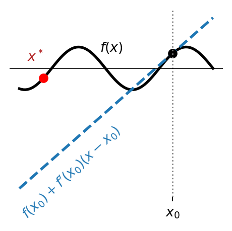
Gauss-Newton is not guaranteed to converge:

  • far from the solution, the linear approximation of \(F\) can be bad enough that the step makes things worse.

Levenberg-Marquardt

Damp with \(\lambda>0\):    \(\mathbf{x} = \mathbf{x}_0 - \big(DF(\mathbf{x}_0)^\top DF(\mathbf{x}_0) + \lambda \mathbf{I}\big)^{-1} DF(\mathbf{x}_0)^\top F(\mathbf{x}_0)\)
  • Small \(\lambda\) \(\to\) behaves like Gauss-Newton;
  • Large \(\lambda\) \(\to\) behaves like a small gradient-descent step.
  • This is exactly the Tikhonov regularization trick applied to the optimization step instead of the least-squares problem.

Demo: Levenberg-Marquardt Rescues a Bad Start

Show code
def levenberg_marquardt(theta0, lam0, max_iter):
    theta = np.array(theta0, dtype=float)
    lam = lam0
    cur = loss(theta)
    hist = [theta.copy()]
    for _ in range(max_iter):
        J, r = jacobian(theta), residual(theta)
        delta = np.linalg.solve(J.T @ J + lam * np.eye(2), -J.T @ r)
        trial = theta + delta
        trial_loss = loss(trial)
        if trial_loss < cur:
            theta, cur, lam = trial, trial_loss, lam * 0.5
        else:
            lam *= 2.0
        hist.append(theta.copy())
    return np.array(hist)

theta0_bad = [0.05, 0.3]
h_gn_bad = gauss_newton(theta0_bad, max_iter=6)
h_lm_bad = levenberg_marquardt(theta0_bad, lam0=1.0, max_iter=30)

losses_gn_bad = np.clip([loss(t) for t in h_gn_bad], None, 1e6)
losses_lm_bad = [loss(t) for t in h_lm_bad]

fig, ax = plt.subplots(figsize=(8.5, 4))
ax.semilogy(range(len(losses_gn_bad)), losses_gn_bad, "-o", color="firebrick", label="Gauss-Newton (undamped)")
ax.semilogy(range(len(losses_lm_bad)), losses_lm_bad, "-o", ms=3, color="steelblue", label="Levenberg-Marquardt")
ax.axhline(loss([a_true, c_true]), color="forestgreen", ls="--", lw=1, label="noise floor")
ax.set_xlabel("iteration $t$"); ax.set_ylabel("$E(\\theta_t)$ (capped at $10^6$ for display)")
ax.set_title(f"Same problem, worse start $(a_0,c_0)=({theta0_bad[0]},{theta0_bad[1]})$", fontsize=10)
ax.legend(fontsize=9)
plt.tight_layout()
plt.show()
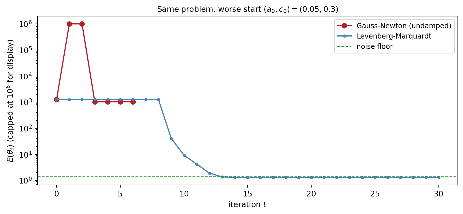
Undamped Gauss-Newton’s first step alone overshoots to a loss above \(10^{40}\) (clipped above for display) and then gets stuck; Levenberg-Marquardt spends a few steps growing \(\lambda\) to stay safe, then shrinks it again and converges cleanly.

Coordinate Descent and Alternation

The Alternation Idea

Suppose \(f(\mathbf{x},\mathbf{y})\) is hard to minimize jointly, but easy to minimize over either variable with the other held fixed.

Alternating optimization

\[ \textbf{for } i=1,2,\dots \qquad \mathbf{x}_{i+1} \leftarrow \min_{\mathbf{x}} f(\mathbf{x},\mathbf{y}_i), \qquad \mathbf{y}_{i+1} \leftarrow \min_{\mathbf{y}} f(\mathbf{x}_{i+1},\mathbf{y}) \]

  • \(f(\mathbf{x}_i,\mathbf{y}_i)\) decreases monotonically: every step is, by definition, a minimization.

But: there is no guarantee of reaching a global (or even local) minimum. Even so, alternation is a great way to turn one hard joint problem into two easy sub-problems, often solvable in closed form.

Example: k-means Clustering as Alternation

k-means objective

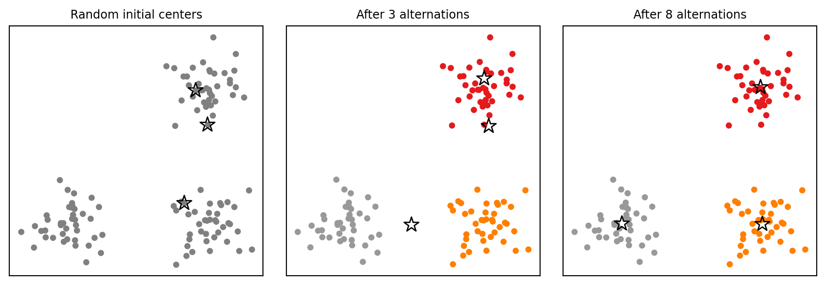
Given data \(\vec{x}_1,\dots,\vec{x}_m\), find \(k\) centers \(\vec{y}_1,\dots,\vec{y}_k\) minimizing \[ E(\vec{y}_1,\dots,\vec{y}_k) \equiv \sum_{i=1}^m \min_{c\in\{1,\dots,k\}} \|\vec{x}_i-\vec{y}_c\|_2^2. \]

Introducing the assignment \(c_i\) explicitly splits the variables into two blocks:

\[\text{labels}\quad \{c_i\}\qquad\qquad\text{centers}\quad\{\vec{y}_j\}.\]

  • Fix centers \(\{\vec{y}_j\}\), optimize labels \(\{c_i\}\): assign each point to its nearest center (closed form).
  • Fix labels \(\{c_i\}\), optimize centers \(\{\vec{y}_j\}\):  \(\vec{y}_j \leftarrow\) mean of the points assigned to cluster \(j\) (closed form).

Example: k-means Clustering as Alternation
def kmeans(X, k, n_iter):
    Y = X[np.random.choice(len(X), k, replace=False)].copy()
    for _ in range(n_iter):
        d2 = ((X[:, None, :] - Y[None, :, :]) ** 2).sum(-1)
        c = d2.argmin(1)                        # assign clusters
        for j in range(k):
            if np.any(c == j):
                Y[j] = X[c == j].mean(0)        # update centers
    return Y, c

Example: Shape Deformation (ARAP)

As-rigid-as-possible (ARAP) deformation

For a mesh with vertices \(v\) and edges \((v,w)\), find rotations \(R_v\) and new positions \(\vec{y}_v\) minimizing \[ \sum_{v}\sum_{(v,w)} \|R_v(\vec{x}_v-\vec{x}_w) - (\vec{y}_v-\vec{y}_w)\|_2^2 \qquad \text{subject to} \quad R_v\in SO(3). \]

  1. Fix \(R_v\), optimize \(\vec{y}_v\):

    A sparse SPD linear system, exactly what conjugate gradient was built for.

  1. Fix \(\vec{y}_v\), optimize \(R_v\):

    Decouples per vertex into a \(2\times2\) closed-form SVD (a rotation-fitting/Procrustes problem).

A hard, nonconvex joint problem, split by alternation into two problems we already know how to solve.

A Quick Tour of More Specialized Tools

Escaping Bad Local Minima

Recall the image-alignment demo:

  • Newton-like local search methods can get stuck in bad local minima due to high-frequency texture in the original images.
  • Blurring the photos first, then sharpening, can avoid bad local alignments caused by fine texture.
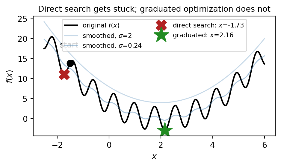
Graduated optimization generalizes this:

  • Solve a sequence \(f_1,f_2,\dots,f_k=f\) of progressively harder problems,
    • using each minimizer as the next initial guess.

The Rest of the Toolbox

Method Idea Use when…
IRLS repeatedly re-weight and re-solve a linear least-squares problem objective like \(\sum_i f_i(\mathbf{x})[g_i(\mathbf{x})]^2\), e.g. \(L^1\)/robust regression
Homotopy continuation continuously morph an easy problem into the hard one related to graduated optimization, framed via topology
Particle swarm / simulated annealing randomized, (mostly) gradient-free global search gradients unavailable or unreliable; many local minima
Online optimization (regret, FTRL) adapt as the objective itself changes over time the objective \(f_t\) changes every iteration (e.g. streaming data)

Rule of thumb: the more specific structure an objective has (sum-of-squares, blocks, convexity), the lighter and faster an algorithm can exploit it.

Looking Ahead

Where These Tools Reappear

  • Numerical/Automatic Differentiation (Classes 10-11): today we hand-derived the Jacobian \(DF(\mathbf{x})\) for Gauss-Newton; you’ll soon compute such derivatives automatically and exactly, for any residual function.
  • ODEs & PDEs (later this semester): implicit time-stepping and constrained field problems often reduce to exactly this kind of alternation or splitting (domain decomposition, operator splitting).
  • Instruments, CAD, 3D printing, and your final projects: fitting a physical model’s parameters to measured data is nonlinear least squares, today’s Gauss-Newton/Levenberg-Marquardt toolkit.

Code Practices

Practice!

Implement Gauss-Newton, Levenberg-Marquardt, and k-means yourself, then play with the interactive demo above:

Open specialized_optimization_demo.ipynb

  • Part 1: Gauss-Newton from scratch, fitting \(y=ce^{ax}\), verified against scipy.optimize.least_squares.
  • Part 2: Levenberg-Marquardt with adaptive damping, from a deliberately bad initial guess.
  • Part 3: k-means from scratch, checking the energy decreases every sub-step.

Recap

Recap on Today’s ILO

  • Explain how Gauss-Newton specializes Newton’s method for sum-of-squares objectives, and implement it, along with Levenberg-Marquardt.
    • Linearizing the residuals turns each step into a linear least-squares problem, no Hessian needed; it converges fast near the solution but is not globally guaranteed. Damping with \(\lambda\) (a Tikhonov-style trick) fixes that.
  • Explain the coordinate descent / alternating optimization strategy, and implement it (k-means).
    • Splitting variables into blocks and minimizing one at a time monotonically decreases the objective; k-means and ARAP both reduce a hard joint problem into closed-form sub-problems.
  • Recognize how global-search heuristics extend these ideas further.
    • Graduated optimization and randomized search address objectives with many local minima.
  • Preview: these tools resurface in automatic differentiation (computing Jacobians), ODE/PDE solvers (splitting), and physical model fitting for instruments, CAD, and final projects.