Interpolation
Topics in Digital Heritage:
Numerical Methods for Digital Reconstruction
Fall 2026
Why Interpolation? Everything Digital Is Sampled
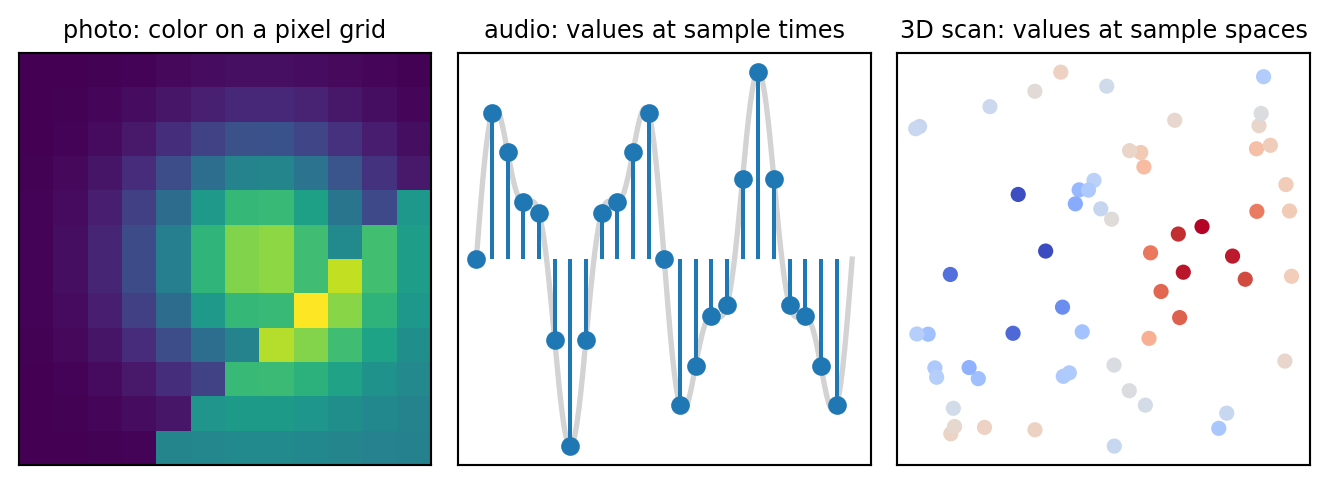
We only know \(f(\mathbf{x}_i)=y_i\) at finitely many \(\mathbf{x}_i\). But, in many scenarios, we need \(f(\mathbf{x})\) between the samples.
(e.g., image rotation, audio fractional delay, surface reconstruction, coordinate transformation, etc.)

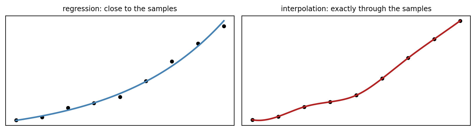
Interpolation problem: given \((\mathbf{x}_1,y_1),\dots,(\mathbf{x}_k,y_k)\), construct \(f\) with \(f(\mathbf{x}_i)=y_i\) that is smooth and adds no spurious features.
Monomial Basis
As one of the simplest basis functions, we can take the monomials \(\phi_i(x)=x^{i-1}\), \(i=1,\dots,k\). With this, \(\boldsymbol{\Phi}\) is the Vandermonde matrix:
\[ \begin{bmatrix} 1 & x_1 & x_1^2 & \cdots & x_1^{k-1}\\ 1 & x_2 & x_2^2 & \cdots & x_2^{k-1}\\ \vdots & & & & \vdots\\ 1 & x_k & x_k^2 & \cdots & x_k^{k-1} \end{bmatrix} \begin{bmatrix} a_0\\ a_1\\ \vdots\\ a_{k-1}\end{bmatrix} = \begin{bmatrix} y_1\\ y_2\\ \vdots\\ y_k\end{bmatrix} \]
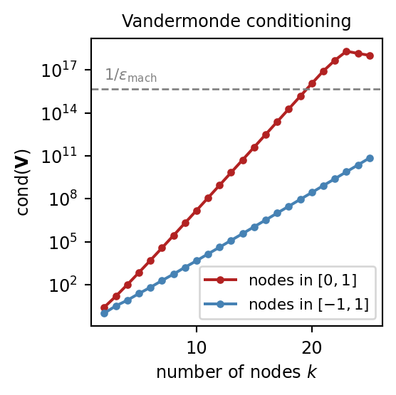
Why Monomials Are a Bad Basis
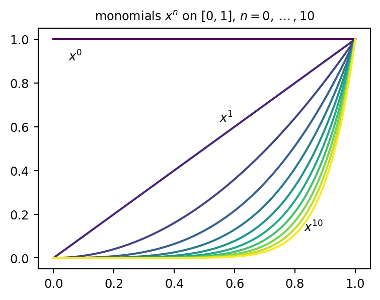
As \(n\) grows, \(x^n\) on \([0,1]\) all look alike.
Measure it with the function inner product \(\langle f,g\rangle=\int_0^1 f(x)g(x)\,dx\): \[ \frac{\langle x^n, x^m\rangle}{\|x^n\|\,\|x^m\|} = \frac{\sqrt{(2n+1)(2m+1)}}{n+m+1}. \] e.g. \(n=9, m=10\), cosine similarity \(\approx 0.997\)
Nearly parallel basis vectors
\(\Rightarrow\) cancelling coefficients in column space
\(\Rightarrow\) ill-conditioned \(\boldsymbol{\Phi}\)
(same lesson as least squares with nearly dependent columns).
Make \(\boldsymbol{\Phi}\) the Identity
Lagrange Basis
\[ \phi_i(x) \equiv \frac{\prod_{j\neq i}(x-x_j)}{\prod_{j\neq i}(x_i-x_j)} \] is \(1\) at its own node and \(0\) at every other node: \[ \phi_i(x_\ell)=\begin{cases}1 & \ell=i\\ 0 & \ell\neq i\end{cases} \] So \(\boldsymbol{\Phi}=\mathbf{I}\) and the coefficients are just the data: \[ f(x)=\sum_i y_i\,\phi_i(x). \] No linear solve at all.
Show code
def lagrange_eval(xk, yk, x):
    """Evaluate the interpolating polynomial in the Lagrange basis."""
    x = np.asarray(x, dtype=float)
    out = np.zeros_like(x)
    for i in range(len(xk)):
        phi = np.ones_like(x)
        for j in range(len(xk)):
            if j != i:
                phi *= (x - xk[j]) / (xk[i] - xk[j])
        out += yk[i] * phi
    return out

xk = np.array([0., 2., 3., 4.])
xs = np.linspace(-0.2, 4.2, 300)
fig, ax = plt.subplots(figsize=(4, 3.3))
for i in range(len(xk)):
    e = np.zeros(len(xk)); e[i] = 1
    ax.plot(xs, lagrange_eval(xk, e, xs), lw=2, label=f"$\\phi_{i+1}$")
ax.plot(xk, np.zeros_like(xk), "ks", ms=4)
ax.plot(xk, np.ones_like(xk), "k.", ms=6)
ax.axhline(0, color="k", lw=0.5); ax.axhline(1, color="gray", lw=0.5, ls=":")
ax.set_ylim(-2, 2)
ax.set_xticks(xk)
ax.set_title("Basis for $0,2,3,4$", fontsize=9)
ax.legend(fontsize=8, ncol=4, loc="upper center")
plt.tight_layout()
plt.show()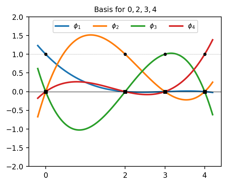
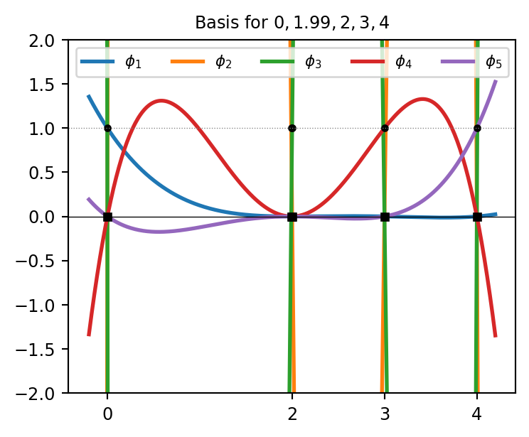
Cost: \(O(k^2)\) per evaluation, and the denominator can be tiny when nodes cluster.
Problem 1: Polynomials Are Nonlocal
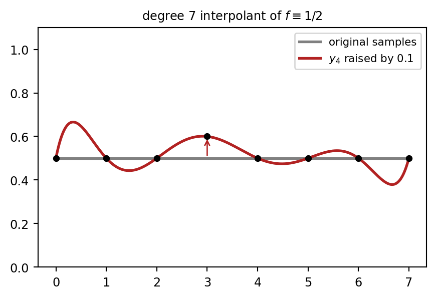
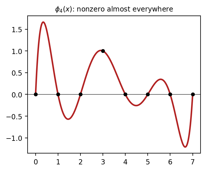
Global support of Lagrange basis functions
Changing one \(y_i\) changes \(f\) everywhere.
Problem 2: The Runge Phenomenon
Simply increasing the number of equispaced nodes can make the interpolant worse (Runge, 1901).
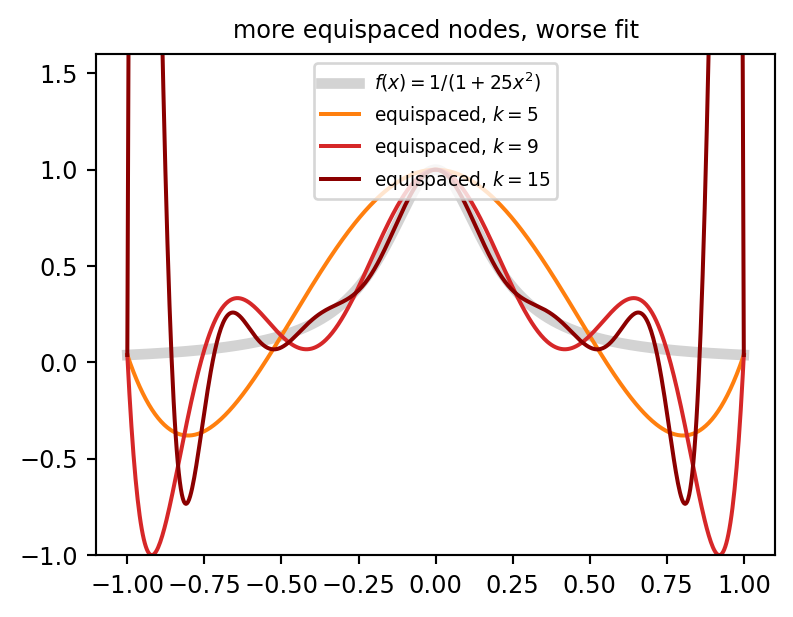
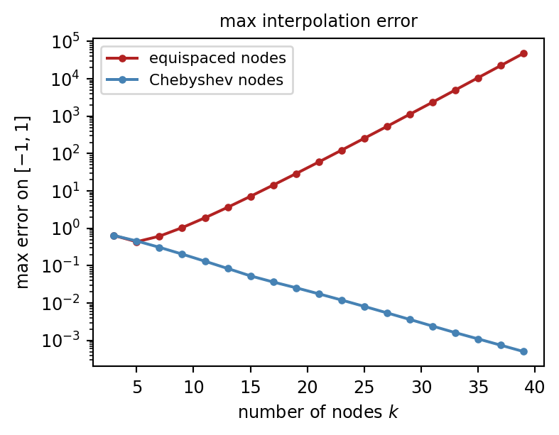
Fix: Use nonuniform nodes (Chebyshev) or piecewise interpolation.
Chebyshev Nodes
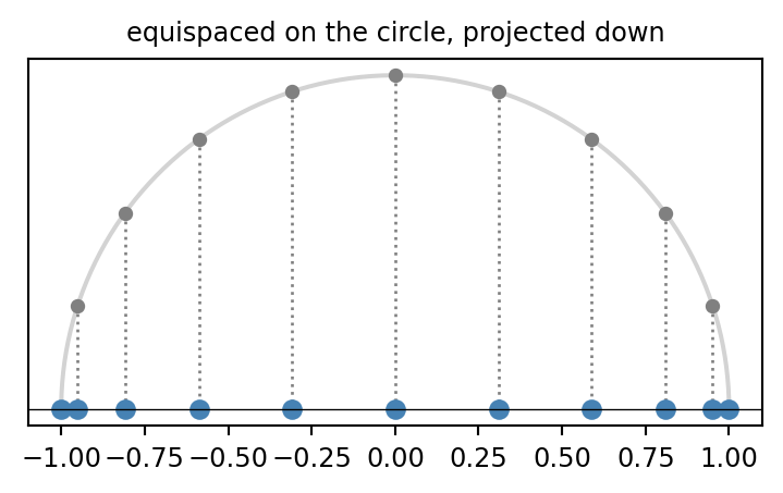
\[x_i = \cos\!\Big(\frac{i\pi}{k-1}\Big),\quad i=0,\dots,k-1\]
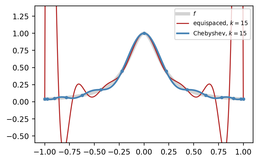
Catch: only possible when we choose where to sample.
But: most of our data (graphics, audio, simulation) is on a fixed grid.
Compact Support: Only Neighbors Matter
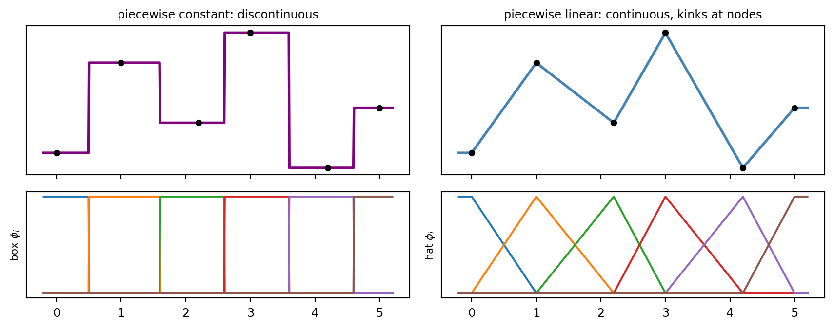
Piecewise constant (nearest neighbor): \[f(x)=y_i,\quad i=\arg\min_j |x-x_j|.\]
Piecewise linear: for \(x\in[x_i,x_{i+1}]\), with \(t=\frac{x-x_i}{x_{i+1}-x_i}\), \[f(x) = (1-t)\,y_i + t\,y_{i+1}.\]
Smoother Pieces: Cubic Splines
| Pieces | Continuity |
|---|---|
| constant | discontinuous |
| linear | \(C^0\) |
| quadratic | up to \(C^1\) |
| cubic | up to \(C^2\) |
Cubic spline: cubic on each interval, matching \(f\), \(f'\), \(f''\) at the nodes. The unknown \(f''(x_i)\) satisfy a tridiagonal system, solvable in \(O(k)\).
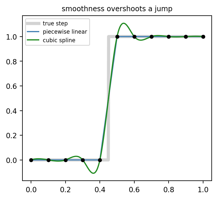
More smoothness = a stronger assumption on \(f\). Discontinuities (edges, shocks) get overshoot.
Application: Fractional Delay in Audio
Show code
fs, D = 48000, 10.37
n = np.arange(2048)
freqs = np.geomspace(100, 16000, 30)

def linear_delay(x, D):                    # 2-tap linear
    m = np.arange(len(x)) - D              # fractional read positions
    return np.interp(m, np.arange(len(x)), x)

def lagrange3(x, D):                       # 4-tap cubic Lagrange
    i0 = int(np.floor(D)) - 1; d = D - i0  # taps at offsets i0..i0+3
    taps = [np.prod([(d - j) / (i - j) for j in range(4) if j != i]) for i in range(4)]
    y = np.zeros_like(x)
    for i, h in enumerate(taps):
        y[i0 + i:] += h * x[:len(x) - i0 - i]
    return y

err_lin, err_lag = [], []
for f0 in freqs:
    x = np.sin(2 * np.pi * f0 * n / fs)
    ref = np.sin(2 * np.pi * f0 * (n - D) / fs)
    s = slice(64, -64)
    err_lin.append(np.abs(linear_delay(x, D) - ref)[s].max())
    err_lag.append(np.abs(lagrange3(x, D) - ref)[s].max())

fig, ax = plt.subplots(figsize=(4.6, 3.4))
ax.loglog(freqs, err_lin, "-o", ms=3, color="steelblue", label="linear (2 taps)")
ax.loglog(freqs, err_lag, "-o", ms=3, color="forestgreen", label="cubic Lagrange (4 taps)")
ax.set_xlabel("frequency [Hz]"); ax.set_ylabel("max error (unit sine)")
ax.set_title(f"delay by D = {D} samples at {fs//1000} kHz", fontsize=9)
ax.legend(fontsize=8)
plt.tight_layout()
plt.show()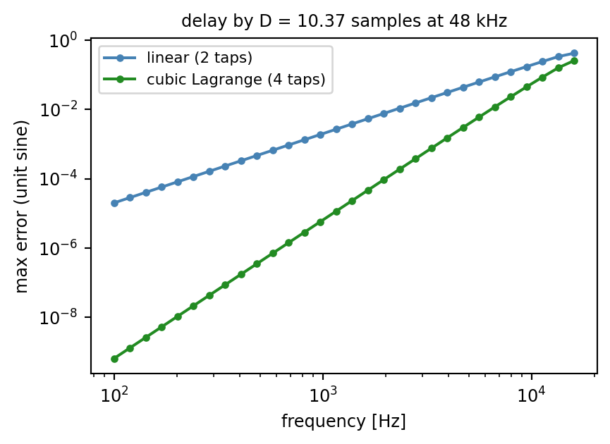

Delay a signal by \(D\) samples: \[y[n] = x[n-D]\]
- Integer \(D\): just shift the array.
- \(D = 10.37\): we must read between samples, i.e., interpolate.
Used in chorus/flanger effects, Doppler, sample-rate conversion, and digital waveguide-ish string and wind models (later this semester), where the delay length sets the pitch.
Nearest Neighbor and Voronoi Cells
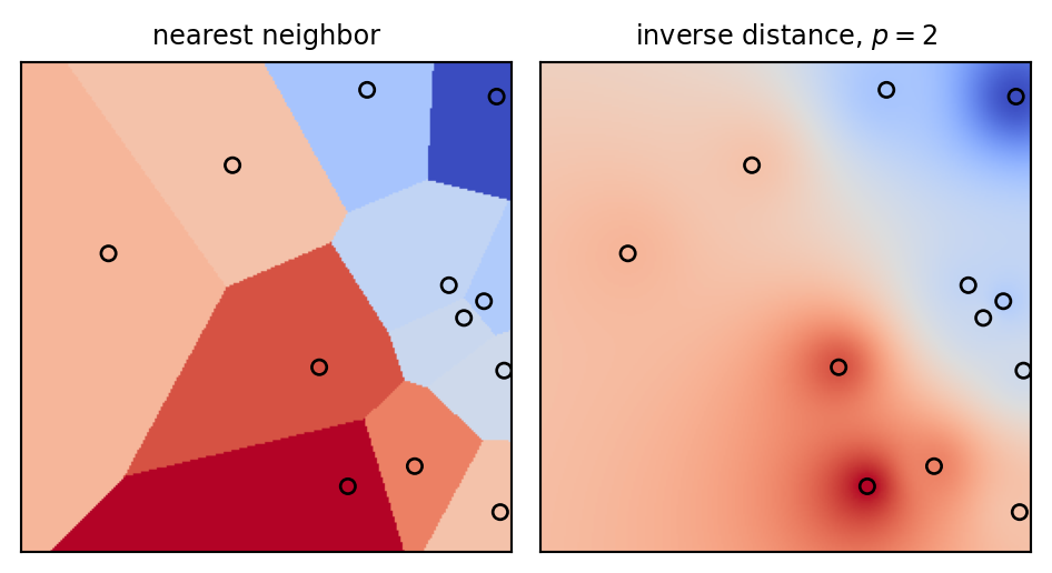
Nearest neighbor: \(f(\mathbf{x}) = y_i\) with \(i=\arg\min_j\|\mathbf{x}-\mathbf{x}_j\|_2\).
Piecewise constant on Voronoi cells \[V_i=\{\mathbf{x}: \|\mathbf{x}-\mathbf{x}_i\|<\|\mathbf{x}-\mathbf{x}_j\|\ \forall j\ne i\}.\]
Fast lookup with a k-d tree (scipy.spatial.cKDTree).
Inverse distance weighting gives a continuous result: \[ f(\mathbf{x}) = \frac{\sum_i w_i(\mathbf{x})\,y_i}{\sum_i w_i(\mathbf{x})},\qquad w_i(\mathbf{x}) = \|\mathbf{x}-\mathbf{x}_i\|_2^{-p}. \] As \(p\to\infty\) it becomes nearest neighbor again.
Barycentric Interpolation on a Triangle
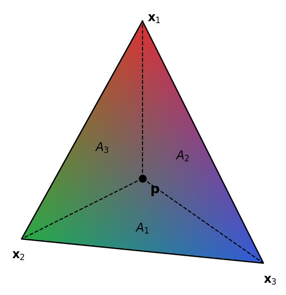
- \(\mathbf{p}\) inside \(\iff\) all \(a_i\ge 0\).
Write \(\mathbf{p}\) as a weighted average of the vertices: \[ \mathbf{p} = a_1\mathbf{x}_1 + a_2\mathbf{x}_2 + a_3\mathbf{x}_3,\quad a_1+a_2+a_3 = 1 \] then interpolate \(f(\mathbf{p}) = a_1y_1+a_2y_2+a_3y_3\).
\(y_i\) can be color, normal, texture coordinate, etc.
- Algebra: linear system \[\begin{bmatrix}\mathbf{x}_1 & \mathbf{x}_2 & \mathbf{x}_3\\ 1 & 1 & 1\end{bmatrix}\mathbf{a} = \begin{bmatrix}\mathbf{p}\\ 1\end{bmatrix}.\]
- Geometry: \(a_i = A_i/A\), the area of the sub-triangle opposite \(\mathbf{x}_i\).
- Gouraud shading
- interpolate vertex colors, normals, texture coordinates across the triangle
- GPU does this billions of times per frame
Grid Data: Bilinear Interpolation
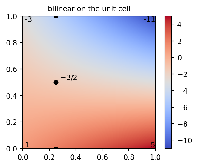
Apply 1D linear interpolation one axis at a time. On a unit cell with \(t_x, t_y\in[0,1]\): \[ \begin{aligned} f(t_x,0) &= (1-t_x)f_{00} + t_x f_{10}\\ f(t_x,1) &= (1-t_x)f_{01} + t_x f_{11}\\ f(t_x,t_y) &= (1-t_y)f(t_x,0) + t_y f(t_x,1) \end{aligned} \]
Example: \(f_{00}=1,\ f_{10}=5,\ f_{01}=-3,\ f_{11}=-11\). Find \(f(\tfrac14,\tfrac12)\): \[ \begin{aligned} f(\tfrac14,0)&=\tfrac34\cdot1+\tfrac14\cdot5=2\\ f(\tfrac14,1)&=\tfrac34(-3)+\tfrac14(-11)=-5\\ f(\tfrac14,\tfrac12)&=\tfrac12\cdot2+\tfrac12(-5)=-\tfrac32 \end{aligned} \] Same answer if you interpolate in \(y\) first.
Code: Rotating an Image with Bilinear Interpolation
Show code
def make_image(n=48):
    u = np.linspace(-1, 1, n)
    X, Y = np.meshgrid(u, u)
    img = ((X**2 + Y**2) < 0.5).astype(float) * 0.7
    img += ((np.abs(X - 0.35) < 0.15) & (np.abs(Y + 0.4) < 0.4)) * 1.0
    img += 0.3 * ((np.floor(4 * (X + 1)) + np.floor(4 * (Y + 1))) % 2)
    return img

def bilinear(img, u, v):
    """Sample img at continuous (row=v, col=u) positions; zero outside."""
    H, W = img.shape
    i0, j0 = np.floor(v).astype(int), np.floor(u).astype(int)
    ty, tx = v - i0, u - j0
    def px(i, j):
        ok = (i >= 0) & (i < H) & (j >= 0) & (j < W)
        return np.where(ok, img[np.clip(i, 0, H - 1), np.clip(j, 0, W - 1)], 0.0)
    top = (1 - tx) * px(i0, j0) + tx * px(i0, j0 + 1)
    bot = (1 - tx) * px(i0 + 1, j0) + tx * px(i0 + 1, j0 + 1)
    return (1 - ty) * top + ty * bot

def nearest(img, u, v):
    return bilinear(img, np.round(u), np.round(v))

def rotate(img, deg, sampler):
    H, W = img.shape
    c = np.array([(H - 1) / 2, (W - 1) / 2])
    I, J = np.mgrid[0:H, 0:W].astype(float)
    th = np.deg2rad(deg)
    # inverse map: for every OUTPUT pixel, where do we read in the INPUT?
    v = np.cos(th) * (I - c[0]) - np.sin(th) * (J - c[1]) + c[0]
    u = np.sin(th) * (I - c[0]) + np.cos(th) * (J - c[1]) + c[1]
    return sampler(img, u, v)

img = make_image()
rep = img.copy()
for _ in range(12):
    rep = rotate(rep, 30, bilinear)

fig, axs = plt.subplots(1, 4, figsize=(9, 2.9))
for ax, im, ttl in zip(axs, [img, rotate(img, 30, nearest), rotate(img, 30, bilinear), rep],
                       ["original", "30°, nearest", "30°, bilinear", "12 × 30° bilinear"]):
    ax.imshow(im, cmap="gray", vmin=0, vmax=2, interpolation="nearest")
    ax.set_title(ttl, fontsize=9); ax.axis("off")
plt.tight_layout()
plt.show()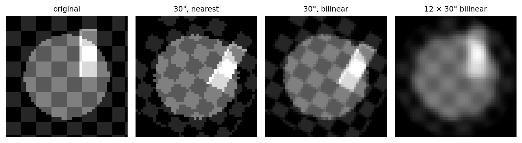
Repeated resampling accumulates blur: compose the transforms, then resample once.