Numerical Integrations
Topics in Digital Heritage:
Numerical Methods for Digital Reconstruction
Fall 2026
Why Integration? Adding Up a Continuum
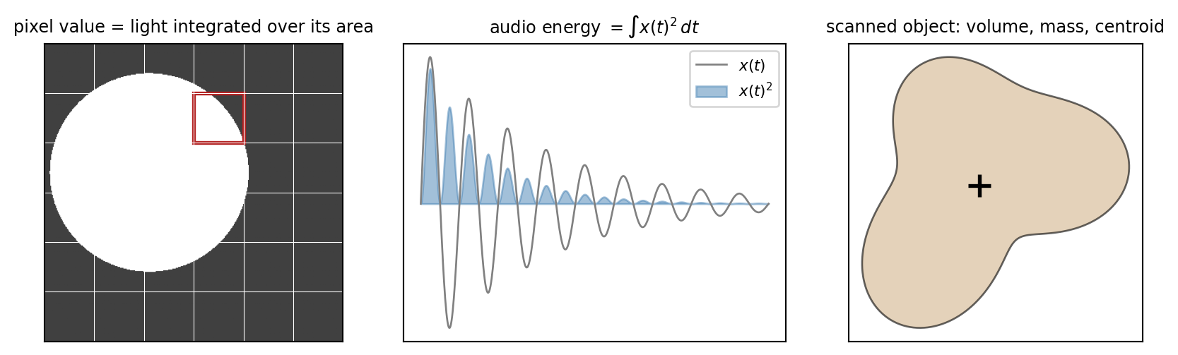
++ light rendering (light arriving from all directions), filter convolution…
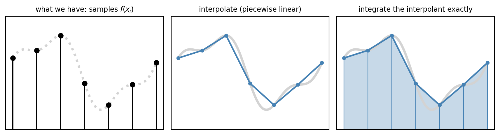
Quadrature problem:
given samples \(f(x_1),\dots,f(x_n)\), approximate \(\displaystyle\int_a^b f(x)\,dx\).
Quadrature Rule = Approximating Integral
Every rule we see today has the same form:
\[ \int_a^b f(x)\,dx \;\approx\; Q[f] \equiv \sum_{i=1}^n w_i\, f(x_i) \]
The Riemann sum from calculus is one example: \(w_i = x_{i+1}-x_i\).
Designing a rule = choosing where to sample (\(x_i\)) with what weight (\(w_i\)).

When samples are given
- recorded audio, camera pixels, scan data, …
- \(x_i\) fixed, we only choose \(w_i\)
When we can evaluate \(f\) anywhere
- ray rendering, simulation, …
- choose \(x_i\) and \(w_i\)
- each evaluation is expensive: accuracy per evaluation matters
Newton-Cotes Rules
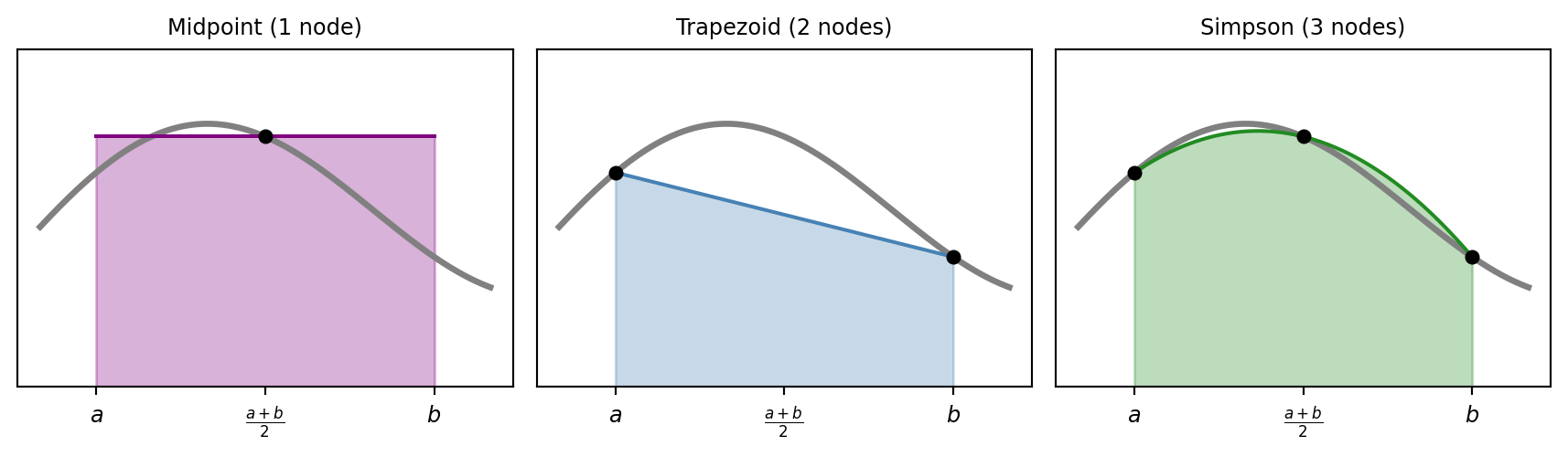
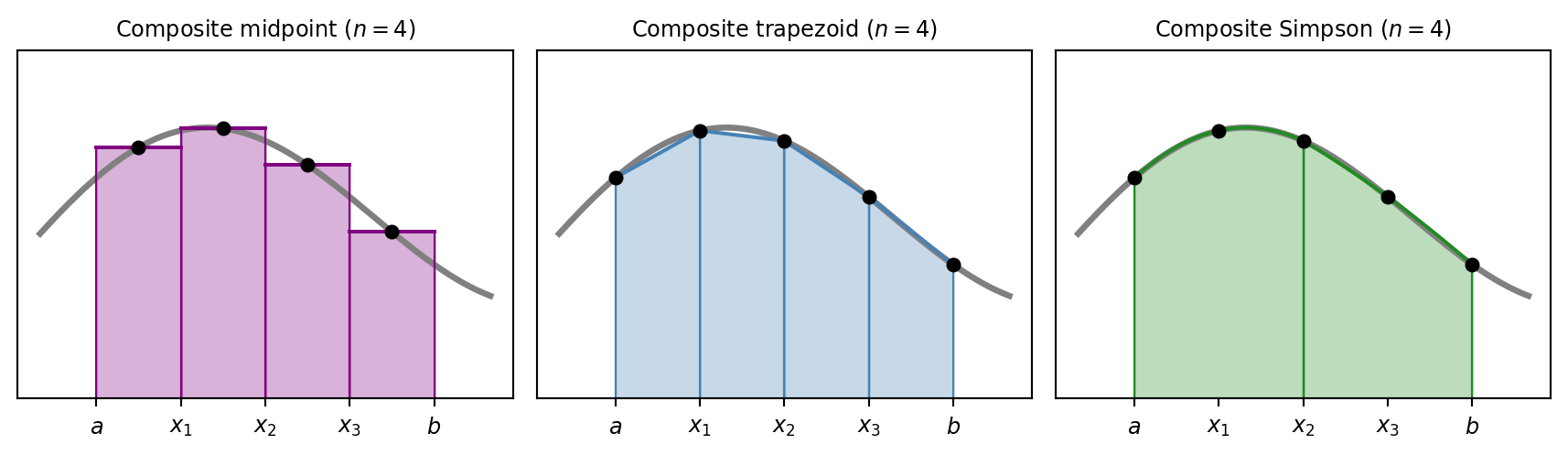
are Quadrature rules that integrate the interpolant on equally spaced nodes.
Midpoint rule
constant interpolant \[(b-a)\,f\!\left(\tfrac{a+b}{2}\right)\]
Trapezoid rule
linear interpolant \[(b-a)\,\frac{f(a)+f(b)}{2}\]
Simpson’s rule
quadratic interpolant \[\frac{b-a}{6}\left[f(a)+4f\!\left(\tfrac{a+b}{2}\right)+f(b)\right]\]
Error on One Interval
Taylor expand \(f\) about the midpoint \(c\) (interval width \(h\)):
\[f(x) = f(c) + f'(c)(x-c) + \frac{1}{2}f''(c)(x-c)^2 + \cdots\]
\[ \begin{aligned} \int_a^b f(x)\,dx &= \int_{-h/2}^{h/2}\left[ f(c) + f'(c) t + \frac{1}{2}f''(c) t^2 + \cdots\right]\,dt\\ &= \underbrace{h\,f(c)}_{\text{midpoint}\\ \equiv\ M} + \underbrace{\frac{h^3}{24}f''(c)}_{\text{error of midpoint}} + O(h^5) \end{aligned} \]
Now Taylor expand the trapezoid rule: \[f(a) = f(c) - \frac{h}{2}f'(c) + \frac{h^2}{8}f''(c) + O(h^3),\quad f(b) = f(c) + \frac{h}{2}f'(c) + \frac{h^2}{8}f''(c) + O(h^3)\] \[ \underbrace{h\,\frac{f(a)+f(b)}{2}}_{\text{trapezoid}\\ \equiv\ T} = h\,f(c) + \frac{h^3}{8}f''(c) + O(h^5),\qquad \int_a^b f(x)\,dx - h\,\frac{f(a)+f(b)}{2} = \underbrace{-\frac{h^3}{12}f''(c)}_{\text{error of trapezoid}} + O(h^5) \]
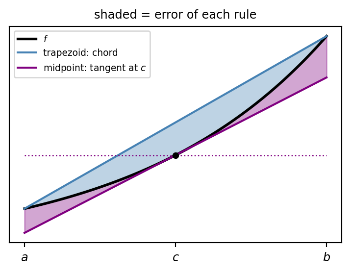
Same order, midpoint error is twice as accurate than trapezoid.
Mix to cancel \(h^3\): \(\ \tfrac{2M+T}{3} = \tfrac{h}{6}\left[f(a)+4f(c)+f(b)\right]\) is Simpson’s rule, error \(O(h^5)\).
Measure the Order of Accuracy
Show code
f = lambda x: np.exp(x) * np.cos(3 * x)                               # smooth, on [0, 2]
F = lambda x: np.exp(x) * (np.cos(3 * x) + 3 * np.sin(3 * x)) / 10    # its antiderivative
exact = F(2.0) - F(0.0)

ns = 2 ** np.arange(1, 13)
h = 2.0 / ns
rules = [("midpoint", midpoint, "purple"), ("trapezoid", trapezoid, "steelblue"), ("Simpson", simpson, "forestgreen")]

fig, axs = plt.subplots(1, 2, figsize=(9, 3.6))
for name, rule, col in rules:
    err = np.array([abs(rule(f, 0, 2, n) - exact) for n in ns])
    p = np.polyfit(np.log(h[2:7]), np.log(err[2:7]), 1)[0]            # slope in the asymptotic range
    axs[0].loglog(h, err, "-o", ms=3, color=col, label=f"{name}: slope {p:.2f}")
axs[0].set_xlabel("sample spacing $h$"); axs[0].set_ylabel("|error|")
axs[0].set_title("three rules, one smooth integrand", fontsize=9)
axs[0].legend(fontsize=8)

# the same rule on three different integrands over [0, 1]
tests = [("smooth: $e^x$", np.exp, np.e - 1, "steelblue"),
         ("kink: $\\sqrt{x}$", np.sqrt, 2 / 3, "firebrick"),
         ("periodic: $e^{\\sin 2\\pi x}$", lambda x: np.exp(np.sin(2 * np.pi * x)), i0(1.0), "darkorange")]
for name, g, ex, col in tests:
    err = np.array([abs(trapezoid(g, 0, 1, n) - ex) for n in ns])
    axs[1].loglog(1.0 / ns, np.maximum(err, 1e-17), "-o", ms=3, color=col, label=name)
axs[1].set_xlabel("sample spacing $h$")
axs[1].set_title("trapezoid rule, three integrands", fontsize=9)
axs[1].legend(fontsize=8)
plt.tight_layout()
plt.show()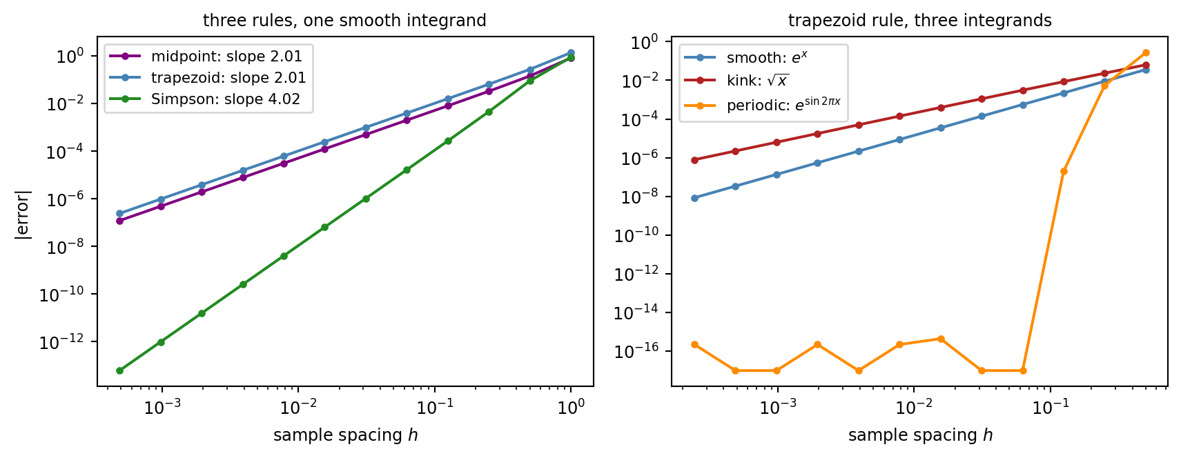
Error \(\approx C h^p\) is a straight line of slope \(p\) on log-log axes.
Always check the slope: a wrong slope means a bug or a non-smooth \(f\).
Gaussian Quadrature
Free the nodes: \(2n\) unknowns (\(x_i\) and \(w_i\))
\(\Rightarrow\) exact for poly up to degree \(2n-1\).
Example: integrate \(f(x)\) using \(n=2\) on \([-1,1]\)
Gaussian quadrature with 2 nodes \[\int_{-1}^{1} f(x)\,dx \approx w_1 f(x_1) + w_2 f(x_2)\tag{$\star$}\]
\(4=2n\) unknowns (\(w_1, w_2, x_1, x_2\)),
can be exact upto degree \(3=2n-1\) (\(1, x, x^2, x^3\))
Set \(f(x) = 1, x, x^2, x^3\) and solve for \(w_i\) and \(x_i\) on \((\star)\):
\[ \begin{aligned} w_1+w_2&=2, & w_1x_1+w_2x_2&=0,\\ w_1x_1^2+w_2x_2^2&=\tfrac23, & w_1x_1^3+w_2x_2^3&=0 \end{aligned} \] \(\Rightarrow\ w_1=w_2=1,\quad x_{1,2}=\mp\tfrac{1}{\sqrt3}\).
Show code
def gauss(f, a, b, n):
    t, w = np.polynomial.legendre.leggauss(n)
    return 0.5 * (b - a) * np.dot(w, f(0.5 * (b - a) * t + 0.5 * (a + b)))

n_tr = 2 ** np.arange(1, 8)
n_ga = np.arange(1, 17)
fig, ax = plt.subplots(figsize=(4.4, 3.3))
ax.loglog(n_tr + 1, [abs(trapezoid(f_test, 0, 2, n) - I_test) for n in n_tr],
          "-o", ms=3, color="steelblue", label="composite trapezoid")
ax.loglog(n_tr + 1, [abs(simpson(f_test, 0, 2, n) - I_test) for n in n_tr],
          "-o", ms=3, color="forestgreen", label="composite Simpson")
ax.loglog(n_ga, [max(abs(gauss(f_test, 0, 2, n) - I_test), 1e-17) for n in n_ga],
          "-o", ms=3, color="firebrick", label="Gaussian, $n$ nodes")
ax.set_xlabel("number of evaluations of $f$"); ax.set_ylabel("|error|")
ax.set_title("$\\int_0^2 e^x\\cos 3x\\,dx$", fontsize=9)
ax.legend(fontsize=7, loc="lower left")
plt.tight_layout()
plt.show()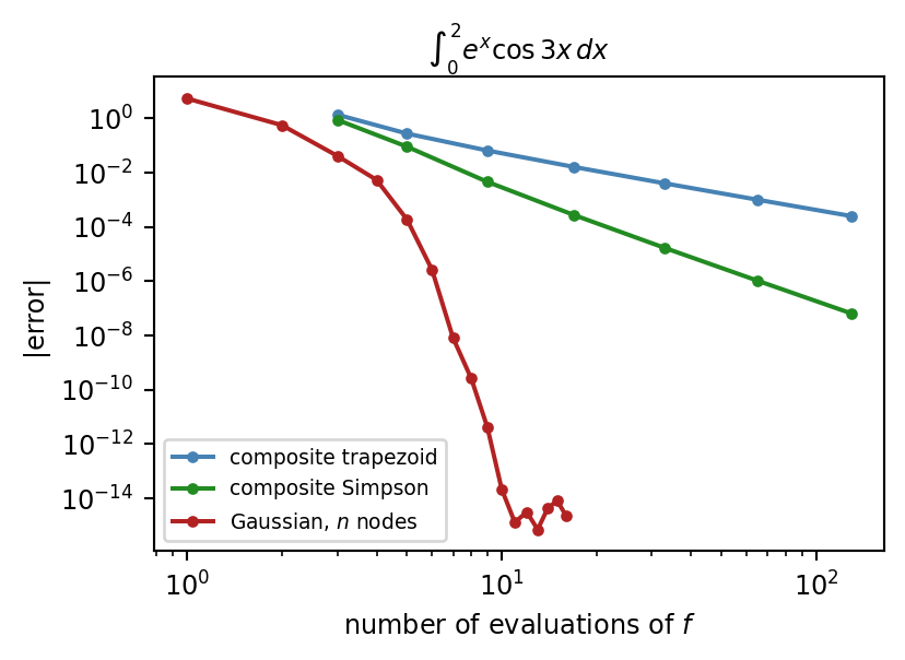
Catch:
- needs \(f\) at prescribed points (not for given samples)
- nodes change completely with \(n\) (no reuse)
- \(f\) must be smooth.
Adaptive Quadrature
Use the function values to decide where more samples are needed.
Error estimate without knowing the answer: compute the integral twice, coarse and fine. If they agree, accept. If not, split the interval and recurse.
def simpson1(f, a, b):       # one Simpson panel
    c = (a + b) / 2
    return (b - a) / 6 * (f(a) + 4 * f(c) + f(b))

def adaptive(f, a, b, tol):
    c = (a + b) / 2
    coarse = simpson1(f, a, b)
    fine = simpson1(f, a, c) + simpson1(f, c, b)
    if abs(fine - coarse) < 15 * tol:
        return fine
    return (adaptive(f, a, c, tol / 2)
            + adaptive(f, c, b, tol / 2))
In practice: cap the recursion depth, or call scipy.integrate.quad(f, a, b).
Show code
s, x0 = 0.02, 1 / np.pi               # a sharp peak of width s at x0
peak = lambda x: np.exp(-np.abs(x - x0) / s)
I_peak = s * (2 - np.exp(-x0 / s) - np.exp(-(1 - x0) / s))

def simpson1(f, a, b):
    return (b - a) / 6 * (f(a) + 4 * f((a + b) / 2) + f(b))

def adaptive(f, a, b, tol, nodes, depth=0):
    c = (a + b) / 2
    coarse, fine = simpson1(f, a, b), simpson1(f, a, c) + simpson1(f, c, b)
    if abs(fine - coarse) < 15 * tol or depth > 30:
        nodes.update([a, (a + c) / 2, c, (c + b) / 2, b])    # points this panel used
        return fine
    return adaptive(f, a, c, tol / 2, nodes, depth + 1) + adaptive(f, c, b, tol / 2, nodes, depth + 1)

nodes = set()
Q = adaptive(peak, 0.0, 1.0, 1e-7, nodes)
err_adaptive = abs(Q - I_peak)

n_uniform = 2                         # how many uniform samples reach the same error?
while abs(simpson(peak, 0, 1, n_uniform) - I_peak) > err_adaptive:
    n_uniform += 2

xs = np.linspace(0, 1, 800)
xa = np.array(sorted(nodes))
fig, ax = plt.subplots(figsize=(4.4, 3.6))
ax.plot(xs, peak(xs), color="gray", lw=2)
ax.plot(xa, peak(xa), "o", color="darkorange", ms=3)
ax.plot(xa, np.full_like(xa, -0.06), "|", color="darkorange", ms=10)
ax.set_xlabel("$x$")
ax.set_title(f"adaptive: {len(xa)} sample points, error {err_adaptive:.0e}\n"
             f"uniform Simpson needs {n_uniform + 1} for the same error", fontsize=9)
plt.tight_layout()
plt.show()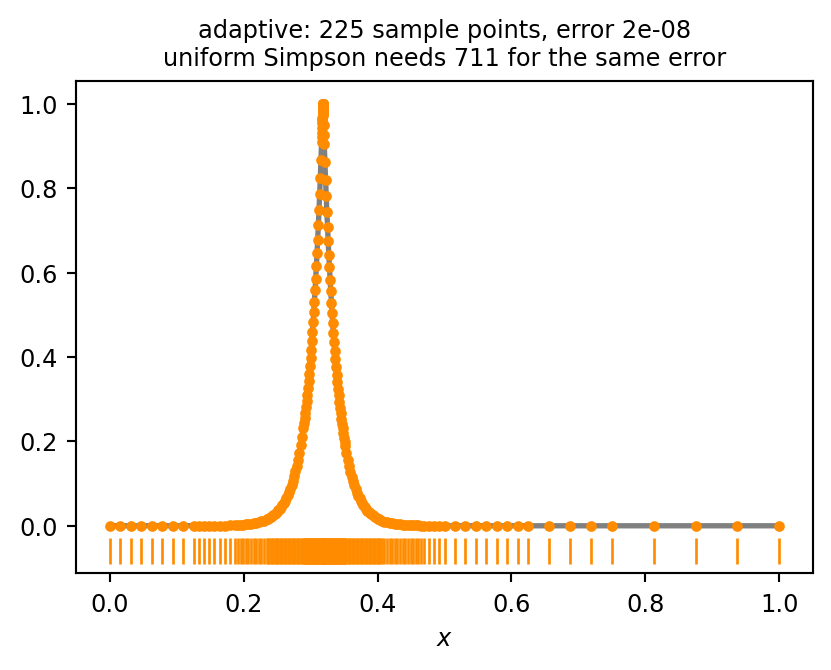
Monte Carlo Integration
Draw \(N\) uniform random points \(\mathbf{x}_i\in\Omega\) and average:
\[ \int_\Omega f(\mathbf{x})\,d\mathbf{x} \approx \frac{\lvert\Omega\rvert}{N}\sum_{i=1}^N f(\mathbf{x}_i) \]
Complicated \(\Omega\)? Sample a bounding box and reject the points outside.
Monte Carlo: Error \(\sim N^{-1/2}\) (independent of \(d\))
Recall: Grid rule had error \(\sim N^{-p/d}\).
Show code
f_d = lambda X: np.exp(X.sum(-1))            # integrate over the unit cube [0, 1]^d
exact_d = lambda d: (np.e - 1) ** d

def grid_midpoint(f, d, n):                  # n^d points, all weights (1/n)^d
    g = (np.arange(n) + 0.5) / n
    X = np.stack(np.meshgrid(*[g] * d, indexing="ij"), -1).reshape(-1, d)
    return f(X).mean()

def mc(f, d, N):
    return f(rng.random((N, d))).mean()

fig, ax = plt.subplots(figsize=(4.6, 4))
for d, n_axis, col in [(2, [3, 10, 32, 100, 316, 1000], "steelblue"), (8, [2, 3, 4, 5, 6], "firebrick")]:
    N = np.array(n_axis) ** d
    e_grid = [abs(grid_midpoint(f_d, d, n) / exact_d(d) - 1) for n in n_axis]
    e_mc = [np.sqrt(np.mean([(mc(f_d, d, n) / exact_d(d) - 1) ** 2 for _ in range(6)])) for n in N]
    ax.loglog(N, e_grid, "-o", ms=4, color=col, label=f"grid midpoint, $d={d}$")
    ax.loglog(N, e_mc, "--s", ms=4, color=col, label=f"Monte Carlo, $d={d}$")
ax.set_xlabel("total number of samples $N$"); ax.set_ylabel("relative error")
ax.set_title("$\\int_{[0,1]^d} e^{x_1+\\cdots+x_d}\\,d\\mathbf{x}$", fontsize=9)
ax.legend(fontsize=7)
plt.tight_layout()
plt.show()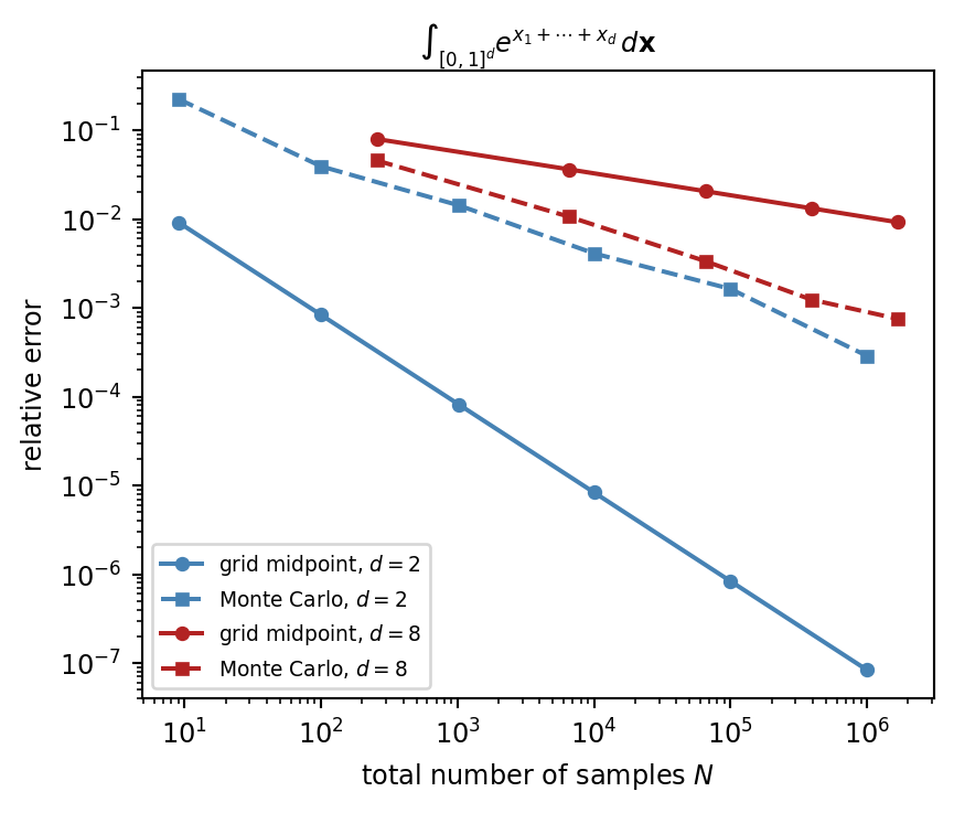
Monte Carlo wins when \(d>2p\).
Monte Carlo Path Tracing


Application: Finite Element Model of a Violin Plate
Goal: predict the vibration modes (Chladni patterns) of a violin top plate, modeled as a flat 3 mm spruce plate with free edges.
Finite element method: Write deflection as \(w\approx\sum_j u_j\,\phi_j\) and solve \(K\mathbf{u}=\omega^2 M\mathbf{u}\), where \[K_{ij}=\int_\Omega \boldsymbol\kappa(\phi_i)^{\top} D\,\boldsymbol\kappa(\phi_j)\,dA,\quad M_{ij}=\int_\Omega \rho h\,\phi_i\,\phi_j\,dA,\quad \boldsymbol\kappa(w)=(w_{xx},\,w_{yy},\,2w_{xy}).\]
\(\boldsymbol\kappa\) is the curvature vector, \(D\) is the bending stiffness matrix, \(\rho\) is the density, and \(h\) is the thickness.
Show code
from scipy.interpolate import CubicSpline
from scipy.spatial import Delaunay
from scipy.linalg import eigh
from matplotlib.path import Path
from matplotlib.tri import Triangulation

def violin_mesh(h=0.01):
    # outline: periodic cubic spline through a few hand-picked points (interpolation, last class)
    half = np.array([[0, 0], [45, 3], [85, 18], [103, 50], [102, 85], [86, 118], [64, 145], [55, 172], [58, 200],
                     [72, 228], [83, 258], [82, 288], [68, 320], [40, 345], [0, 356]]) * 1e-3
    ctrl = np.vstack([half, (half * [-1, 1])[-2:0:-1], half[:1]])
    s = np.concatenate([[0], np.cumsum(np.linalg.norm(np.diff(ctrl, axis=0), axis=1))])
    spline = CubicSpline(s, ctrl, bc_type="periodic")
    fine = spline(np.linspace(0, s[-1], 4000, endpoint=False))
    arc = np.concatenate([[0], np.cumsum(np.linalg.norm(np.diff(fine, axis=0), axis=1))])
    nb = int(arc[-1] / h)
    bnd = np.stack([np.interp(np.arange(nb) * arc[-1] / nb, arc, fine[:, k]) for k in range(2)], 1)
    # interior: hexagonal lattice, then Delaunay, then drop triangles outside the outline
    gx, gy = np.meshgrid(np.arange(-0.12, 0.12, h), np.arange(0, 0.36, h * np.sqrt(3) / 2))
    gx[1::2] += h / 2
    P = np.stack([gx.ravel(), gy.ravel()], 1)
    keep = Path(bnd).contains_points(P) & (np.linalg.norm(P[:, None] - bnd[None], axis=2).min(1) > 0.7 * h)
    P = np.vstack([bnd, P[keep]])
    T = Delaunay(P).simplices
    T = T[Path(bnd).contains_points(P[T].mean(1))]
    return P, T, bnd

# 6 point Gauss rule on a triangle (exact up to degree 4), in barycentric coordinates
a1, a2, w1, w2 = 0.445948490915965, 0.091576213509771, 0.223381589678011, 0.109951743655322
tri_bary = np.array([[a, a, 1 - 2 * a] for a in (a1, a2)]).repeat(3, 0)
tri_bary = np.array([np.roll(r, k) for r, k in zip(tri_bary, [0, 1, 2] * 2)])
tri_w = np.array([w1] * 3 + [w2] * 3)

mono = lambda X: np.stack([np.ones(len(X)), X[:, 0], X[:, 1], X[:, 0]**2, X[:, 0] * X[:, 1], X[:, 1]**2], 1)
dmono = lambda X: (np.stack([0 * X[:, 0], 1 + 0 * X[:, 0], 0 * X[:, 0], 2 * X[:, 0], X[:, 1], 0 * X[:, 0]], 1),
                   np.stack([0 * X[:, 0], 0 * X[:, 0], 1 + 0 * X[:, 0], 0 * X[:, 0], X[:, 0], 2 * X[:, 1]], 1))

def plate_modes(P, T, D, rho_h, n_modes=4):
    """Free vibration of a thin plate. Quadratic (Morley) elements: unknowns are the
    deflection w at the vertices and the normal slope dw/dn at the edge midpoints."""
    edges = {}
    for tri in T:
        for k in range(3):
            edges.setdefault(tuple(sorted((tri[k - 2], tri[k - 1]))), len(P) + len(edges))
    n = len(P) + len(edges)
    K, M = np.zeros((n, n)), np.zeros((n, n))
    for tri in T:
        X = P[tri] - P[tri].mean(0)
        area = 0.5 * abs(np.linalg.det(X[1:] - X[0]))
        dof, A = list(tri), [mono(X)]
        for k in range(3):                                   # edge opposite to vertex k
            i, j = sorted((tri[k - 2], tri[k - 1]))
            t = (P[j] - P[i]) / np.linalg.norm(P[j] - P[i])
            mid = (0.5 * (P[i] + P[j]) - P[tri].mean(0))[None]
            dx, dy = dmono(mid)
            A.append(t[1] * dx - t[0] * dy)
            dof.append(edges[(i, j)])
        C = np.linalg.inv(np.vstack(A))                      # column j = coefficients of basis function phi_j
        B = np.stack([2 * C[3], 2 * C[5], 2 * C[4]])         # curvatures (w_xx, w_yy, 2 w_xy), constant on the triangle
        Phi = mono(tri_bary @ X) @ C                         # phi_j at the 6 Gauss points
        K[np.ix_(dof, dof)] += area * B.T @ D @ B                        # integral of kappa_i^T D kappa_j
        M[np.ix_(dof, dof)] += rho_h * area * (Phi.T * tri_w) @ Phi      # integral of rho h phi_i phi_j
    lam, U = eigh(K, M, subset_by_index=[0, n_modes + 2])
    return np.sqrt(np.abs(lam[3:])) / (2 * np.pi), U[: len(P), 3:]       # skip the 3 rigid body motions

P, T, outline = violin_mesh()

# spruce, grain along the length (y): bending stiffness matrix D = h^3/12 * Q
E_x, E_y, G, nu_yx, rho, thick = 0.9e9, 11e9, 0.7e9, 0.37, 420.0, 3e-3
c = 1 - nu_yx**2 * E_x / E_y
D = thick**3 / 12 * np.array([[E_x / c, nu_yx * E_x / c, 0], [nu_yx * E_x / c, E_y / c, 0], [0, 0, G]])
freq, modes = plate_modes(P, T, D, rho * thick)

fig, axs = plt.subplots(1, 6, figsize=(9, 2.5), width_ratios=[1, 1.15, 1, 1, 1, 1])
closed = np.vstack([outline, outline[:1]])
axs[0].triplot(P[:, 0], P[:, 1], T, color="steelblue", lw=0.4)
axs[0].plot(closed[:, 0], closed[:, 1], color="k", lw=0.8)
axs[0].set_title(f"{len(T)} triangles", fontsize=9)

e = np.argmin(np.linalg.norm(P[T].mean(1) - [0.0, 0.17], axis=1))       # zoom into one element
X = P[T[e]]
axs[0].fill(X[:, 0], X[:, 1], color="firebrick")
axs[1].fill(X[:, 0], X[:, 1], color="steelblue", alpha=0.15, ec="steelblue")
axs[1].scatter(*(tri_bary @ X).T, s=400 * tri_w, color="firebrick", label="Gauss points")
axs[1].plot(X[:, 0], X[:, 1], "o", color="k", ms=5, label="$w$")
mid = 0.5 * (X + np.roll(X, 1, 0))
axs[1].plot(mid[:, 0], mid[:, 1], "s", color="k", mfc="w", ms=5, label="$\\partial w/\\partial n$")
axs[1].margins(0.2)
axs[1].legend(fontsize=6, loc="upper center", bbox_to_anchor=(0.5, 0.0), ncol=1, frameon=False)
axs[1].set_title("one element", fontsize=9)

tri = Triangulation(P[:, 0], P[:, 1], T)
for k, ax in enumerate(axs[2:]):
    w = modes[:, k] / np.abs(modes[:, k]).max()
    ax.tricontourf(tri, w, levels=np.linspace(-1, 1, 21), cmap="RdBu_r")
    ax.tricontour(tri, w, levels=[0], colors="k", linewidths=1.2)        # nodal lines (Chladni pattern)
    ax.plot(closed[:, 0], closed[:, 1], color="k", lw=0.8)
    ax.set_title(f"mode {k + 1}: {freq[k]:.0f} Hz", fontsize=9)
for ax in axs:
    ax.set_aspect("equal"); ax.axis("off")
for ax in [axs[0], *axs[2:]]:
    ax.set_xlim(-0.115, 0.115); ax.set_ylim(-0.01, 0.366)
plt.tight_layout()
plt.show()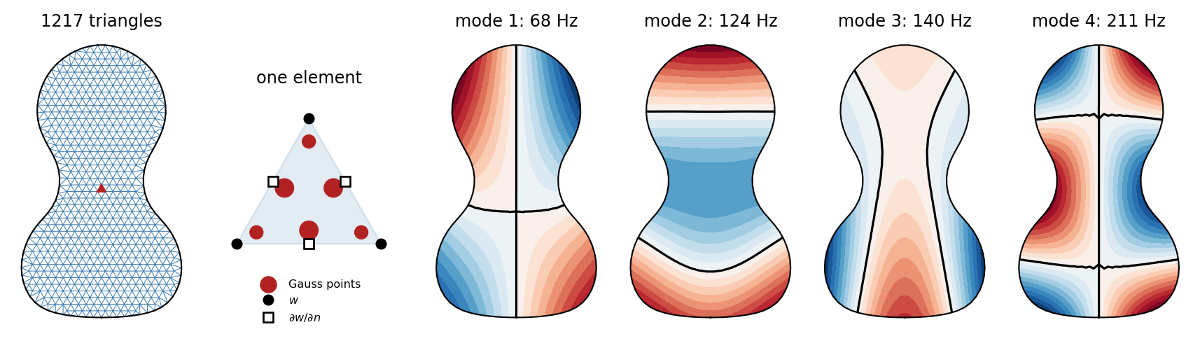
Triangular mesh \(\to\) quadratic basis functions \(\phi_j\) \(\to\) generalized eigenvalue problem \(K\mathbf{u}=\omega^2 M\mathbf{u}\).
Each entry is a sum of triangle integrals \(\int_T g\,dA\approx|T|\sum_q w_q\,g(\mathbf{x}_q)\).
Here \(\phi_i\phi_j\) has degree 4, so a 6 point Gauss rule is exact.