Numerical Study of Air-jet Instrument Sounds using Hydrodynamic-Acoustic Splitting
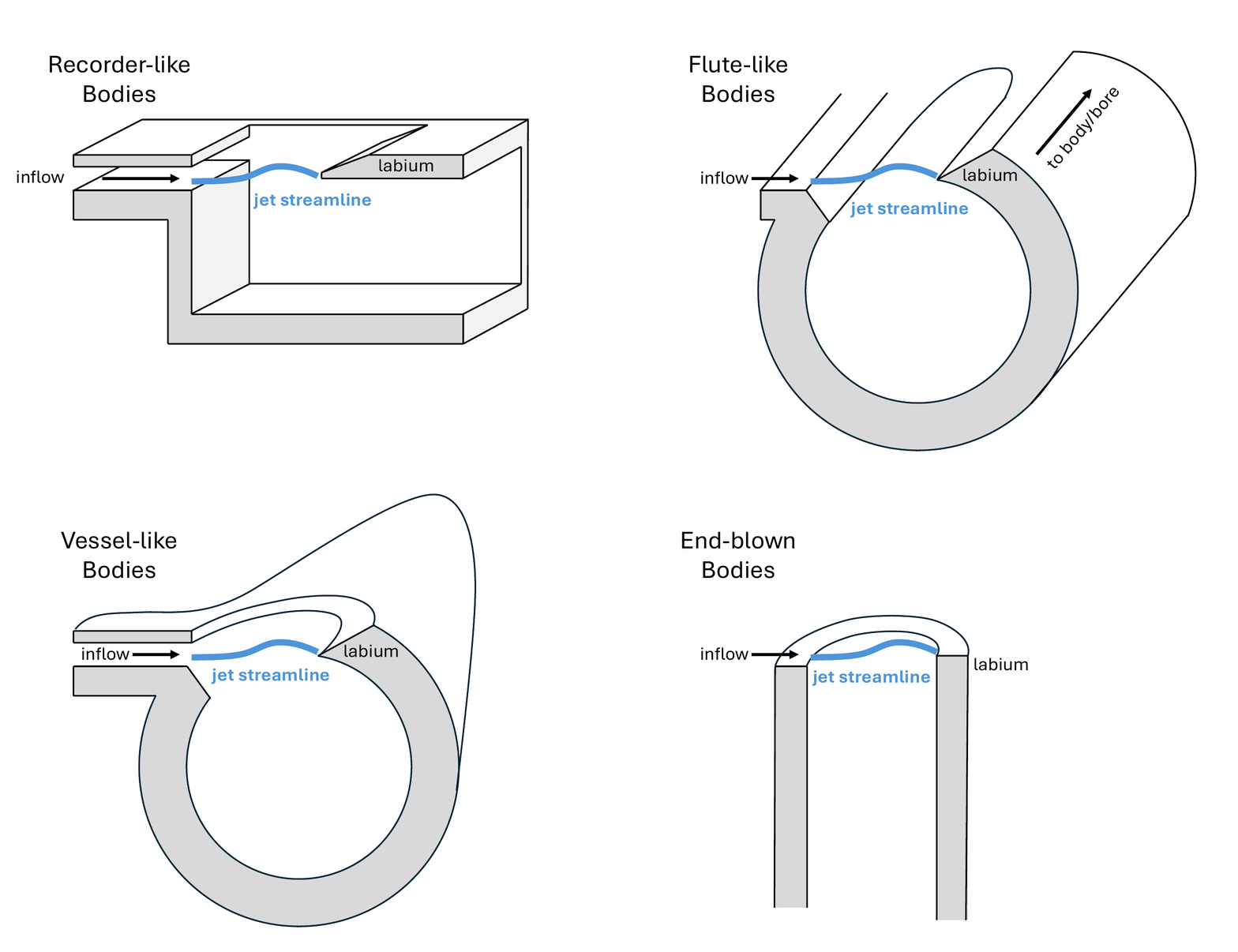
Air-jet Instruments
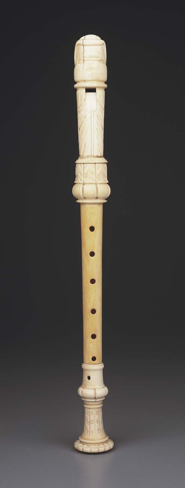
- Recorders
![]() Alto recorder
Alto recorder
[Accession Number 17.1809]
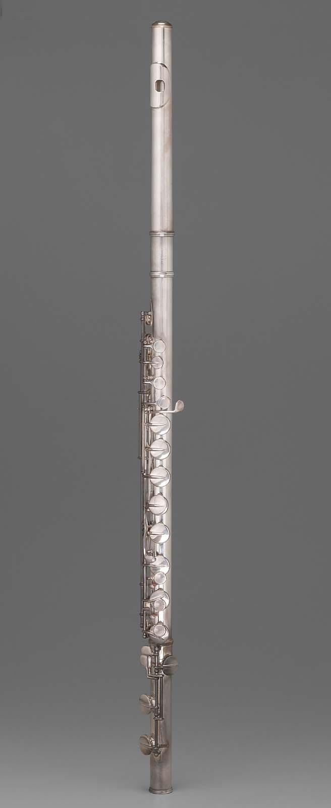
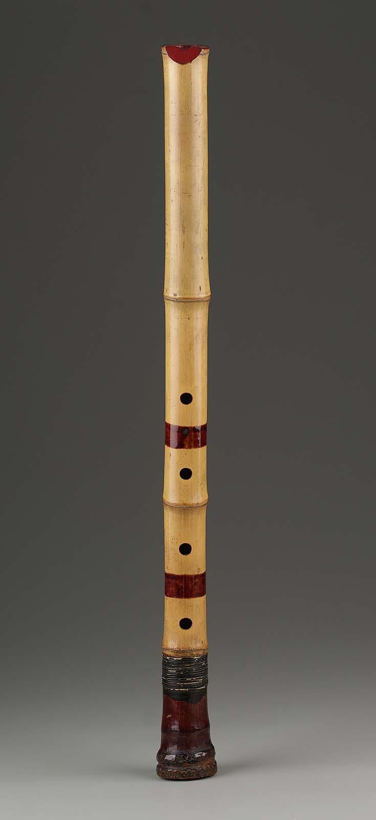
- Flutes
![]()
![]() Alto flute in G (Boehm system) End-blown flute (shakuhachi) [Accession Number 1986.800] [Accession Number 17.2154]
Alto flute in G (Boehm system) End-blown flute (shakuhachi) [Accession Number 1986.800] [Accession Number 17.2154]
- Vessel Flutes
![]() Soprano ocarina
Soprano ocarina
[Accession Number 1984.309]
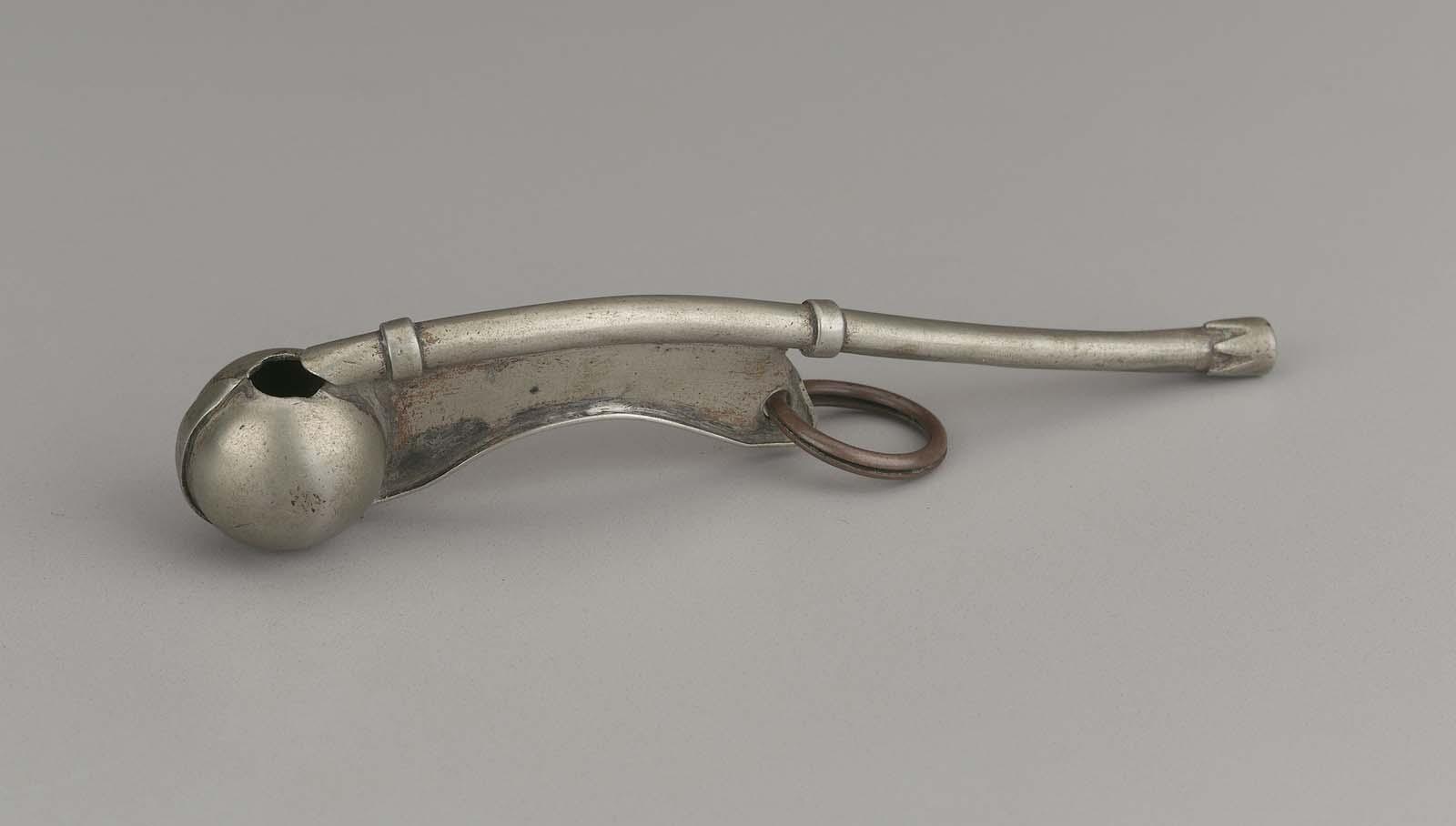
- Whistles
![]() Boatswain’s whistle
Boatswain’s whistle
[Accession Number 17.1830]
All images courtesy of the Museum of Fine Arts, Boston. www.mfa.org
Hydrodynamic-Acoustic Splitting
 \[\underbrace{p(\mathbf{x},t)}_{\mathrm{Total~Pressure}} = \underbrace{P(\mathbf{x},t)}_{\mathrm{Fluid}} + \underbrace{p'(\mathbf{x},t)}_{\mathrm{Acoustic}}\]
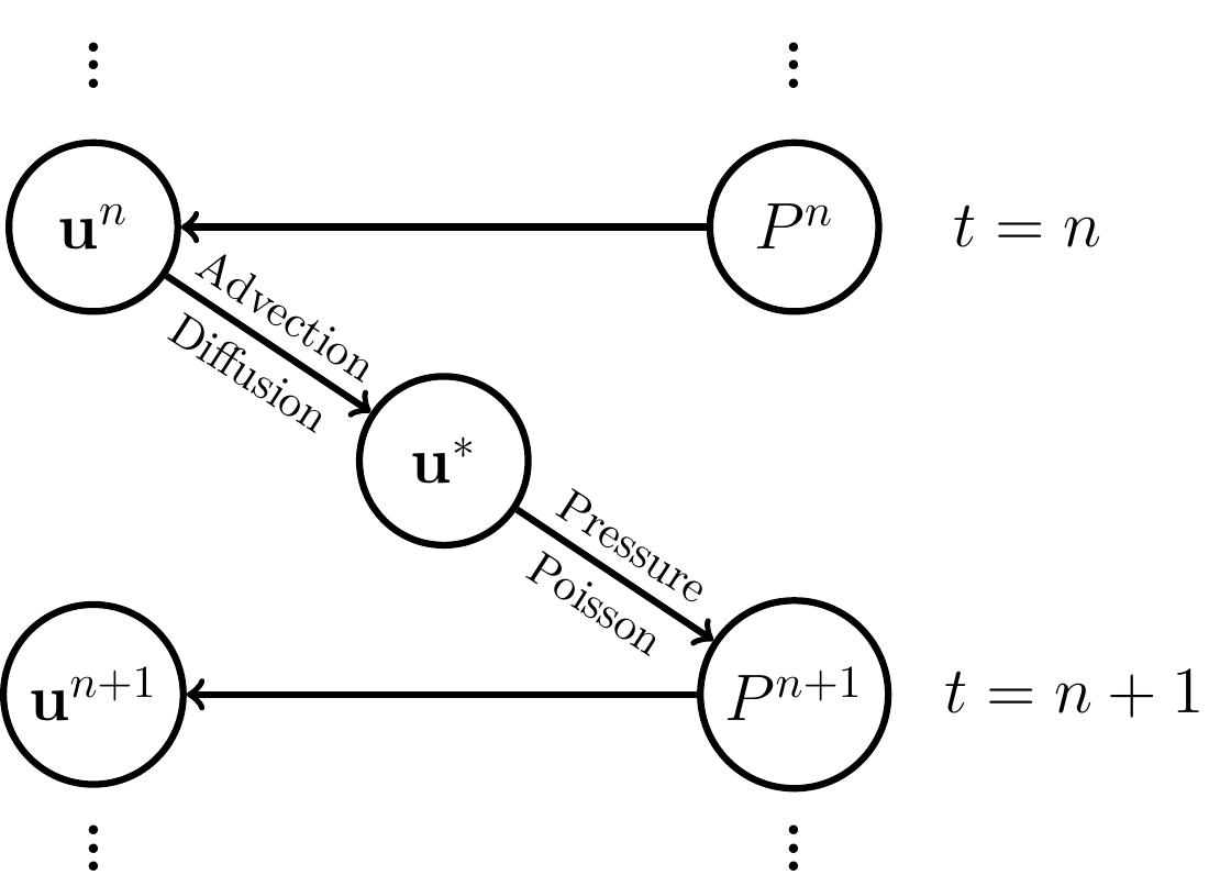
\(P\): incompressible Navier–Stokes
\(p'\): inhomogeneous wave equation
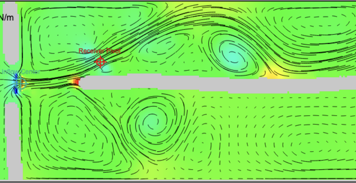
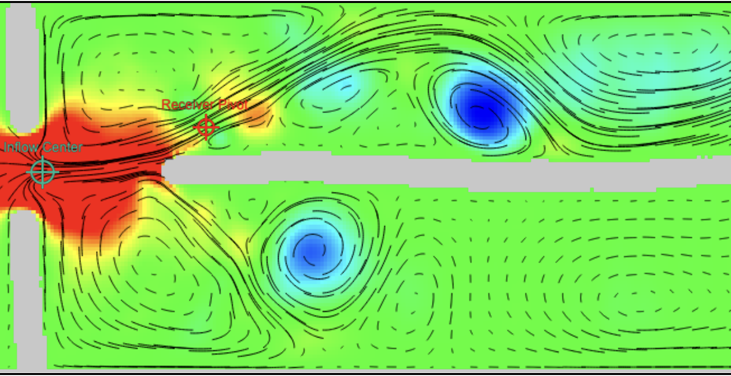
Moving on to the acoustic part…
\[\underbrace{p(\mathbf{x},t)}_{\mathrm{Total~Pressure}} = \underbrace{P(\mathbf{x},t)}_{\mathrm{Fluid}} + \underbrace{p'(\mathbf{x},t)}_{\mathrm{Acoustic}}\]
\(P\): incompressible Navier–Stokes
\(p'\): inhomogeneous wave equation
Acoustic Update Rule
The acoustic field described in an inhomogeneous wave equation: \[\begin{equation} \frac{1}{c_0^2}\,\frac{\partial^2 p'}{\partial t^2} - \Delta p' = \frac{\partial^2 L_{ij}}{\partial x_i\,\partial x_j} \end{equation}\]
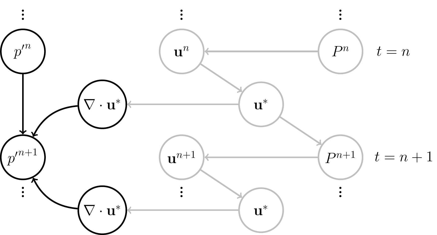
- Störmer–Verlet \[\small\begin{align} {p'}^{n+1} &= 2{p'}^n - {p'}^{n-1} \\ &+ (c_0 T_2)^2\nabla^2{p'}^n + S^n \end{align}\]
- Acoustic source \(\small S^n = -\rho_0\,c_0^2\,\frac{T_2^2}{K\,T_1}\,\bigl(D_{k+1} - D_k\bigr)\) \(\small D = \nabla \cdot \mathbf{u}^*\)
Acoustic Update Rule
The acoustic field described in an inhomogeneous wave equation: \[\begin{equation} \frac{1}{c_0^2}\,\frac{\partial^2 p'}{\partial t^2} - \Delta p' = \frac{\partial^2 L_{ij}}{\partial x_i\,\partial x_j} \end{equation}\]
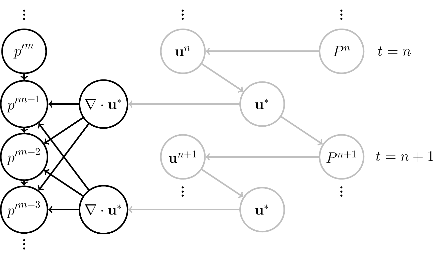
Acoustic time step \[\begin{align} T_2 &= \tfrac{\lambda_2}{\sqrt{3}}\tfrac{X_i}{\color{red}{c_0}} \\ &\approx \color{red}{3.4\times10^{-7}} \end{align}\] \[(c_0=343\ \mathrm{m/s},\ \lambda_2=1.0)\]
Recall: Hydrodynamic time step \[\begin{align} T_1 &= \min\!\left(\tfrac{\lambda_1}{\sqrt{3}}\tfrac{X_i}{\color{red}{U_0}},\;\tfrac{X_i^2}{6\nu}\right) \\ &\approx \color{red}{2.8\times10^{-6}} \end{align}\] \[(U_0\approx17\ \mathrm{m/s},\ \lambda_1=0.4)\]
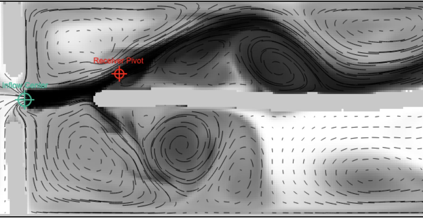
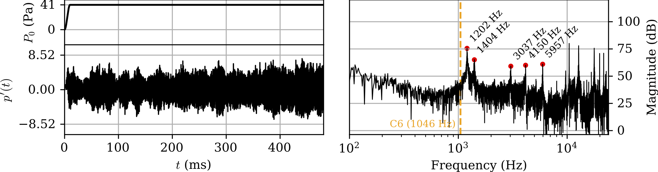
Result: Tenor Recorder
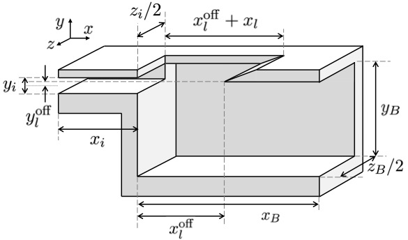
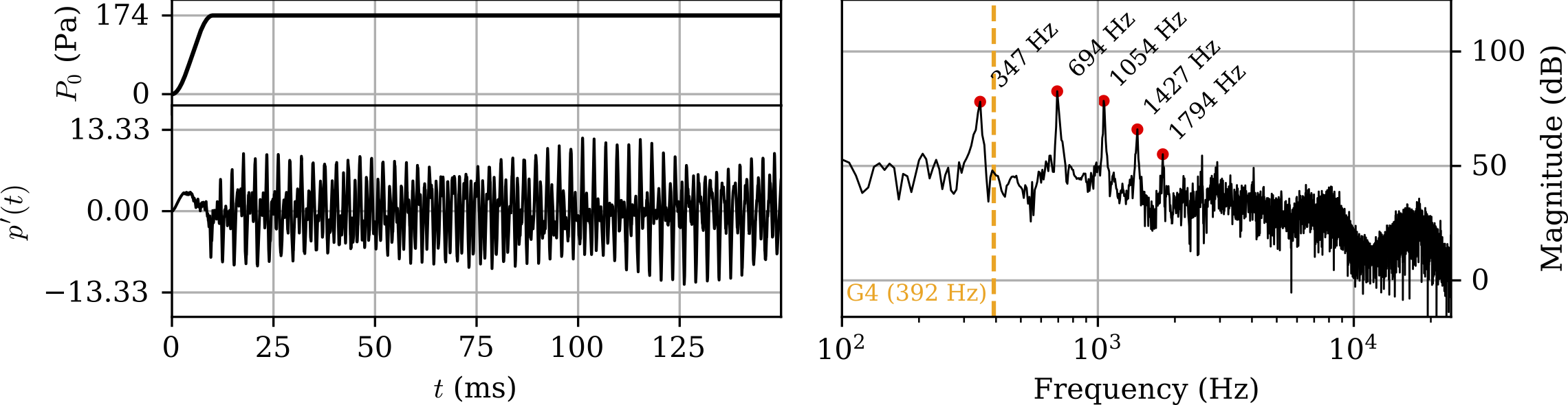
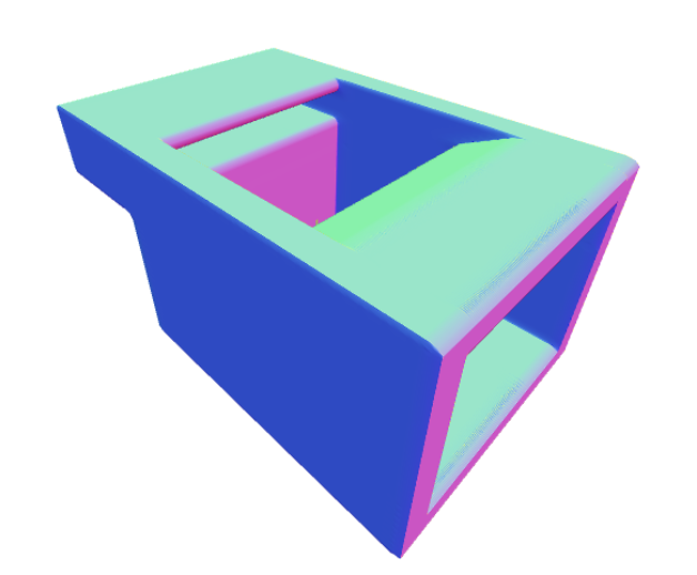
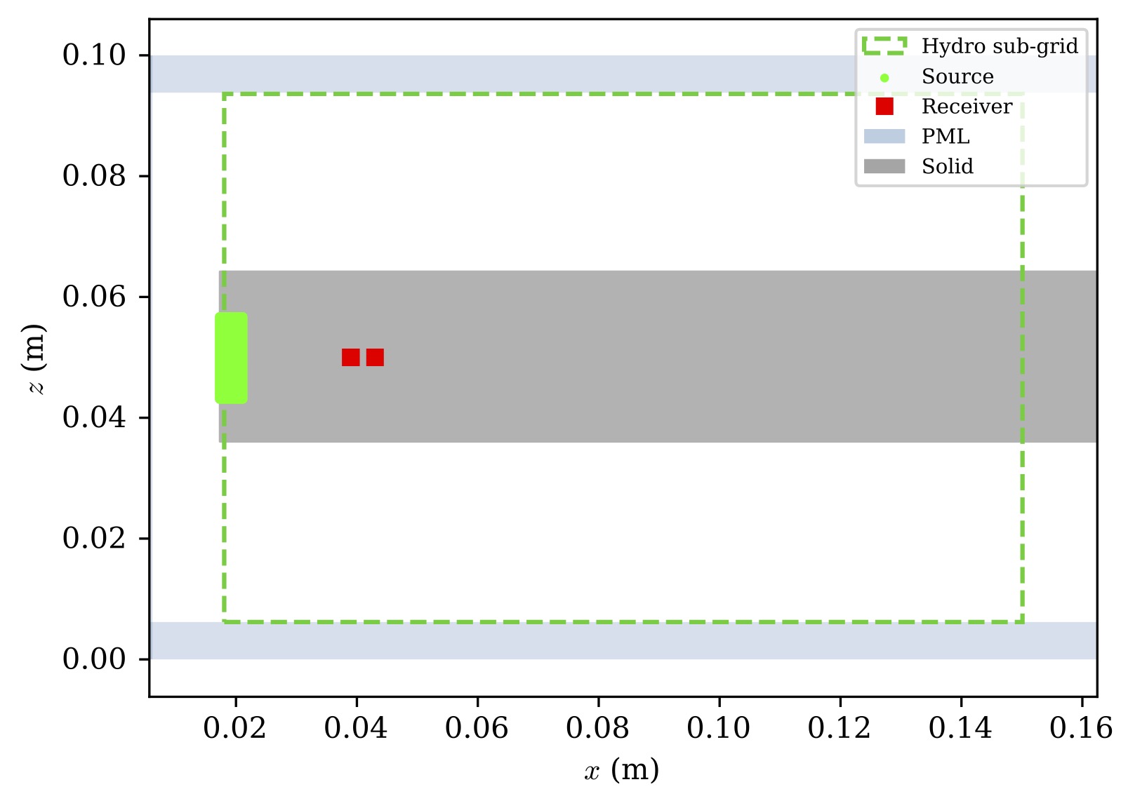
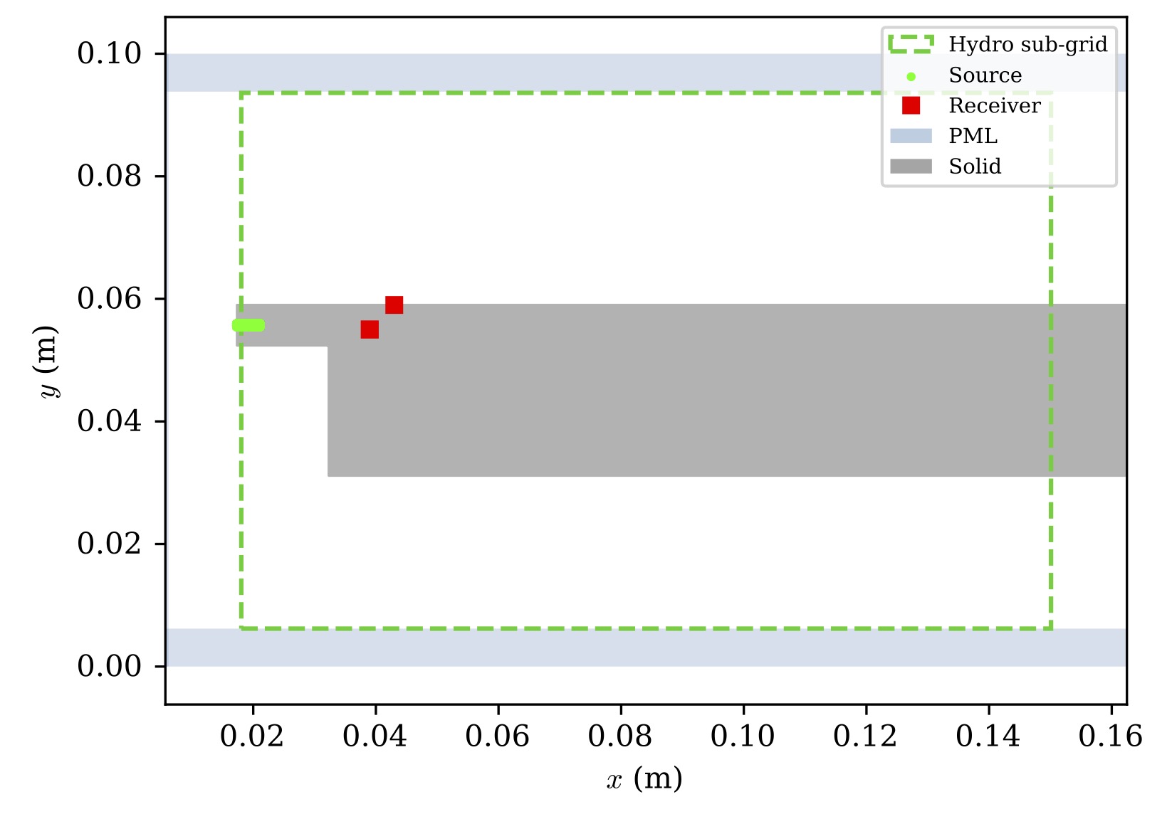
Result: Historic Vessel Flute
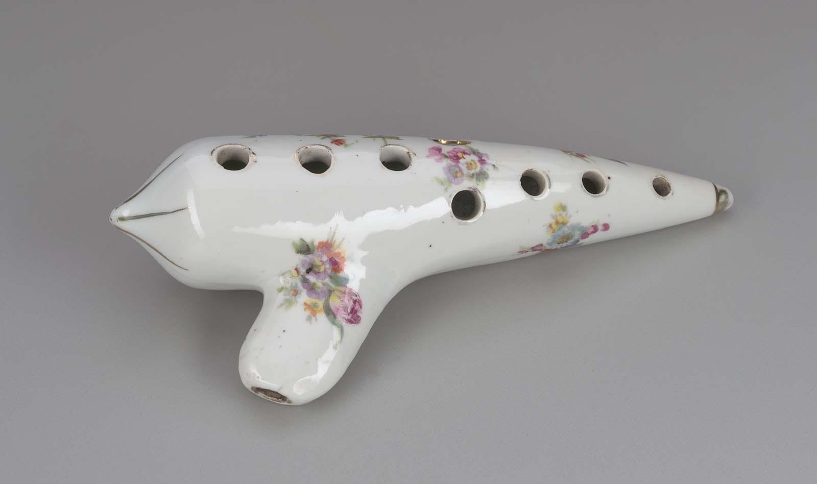
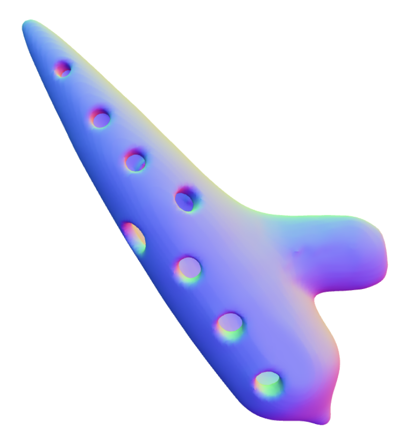
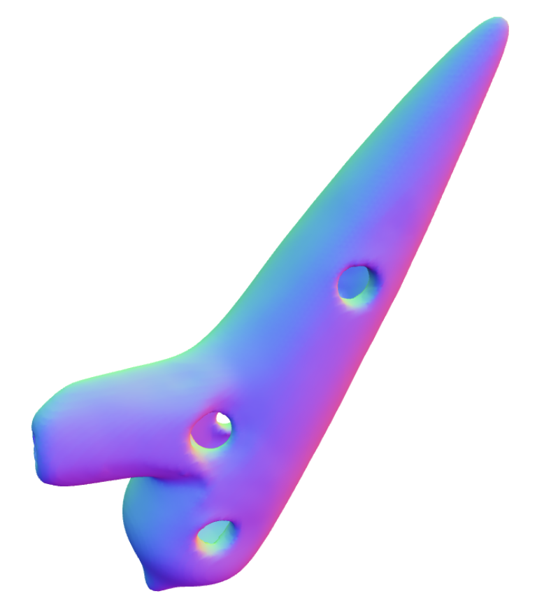
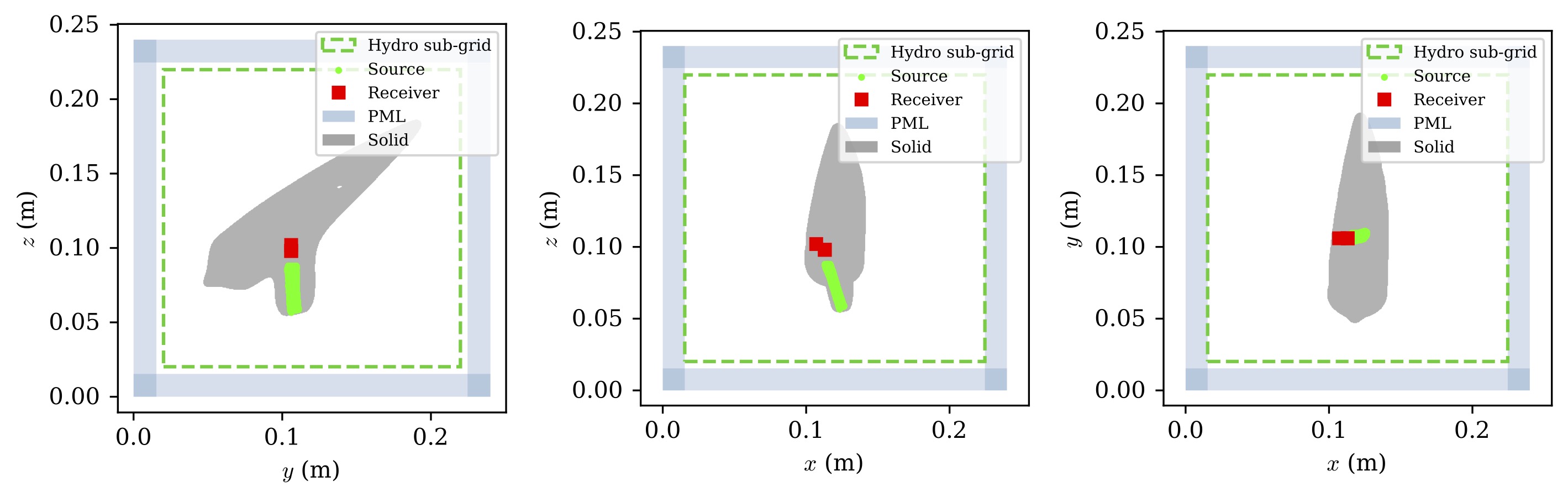
Soprano ocarina photo courtesy of the Museum of Fine Arts, Boston. www.mfa.org
Result: Historic Vessel Flute
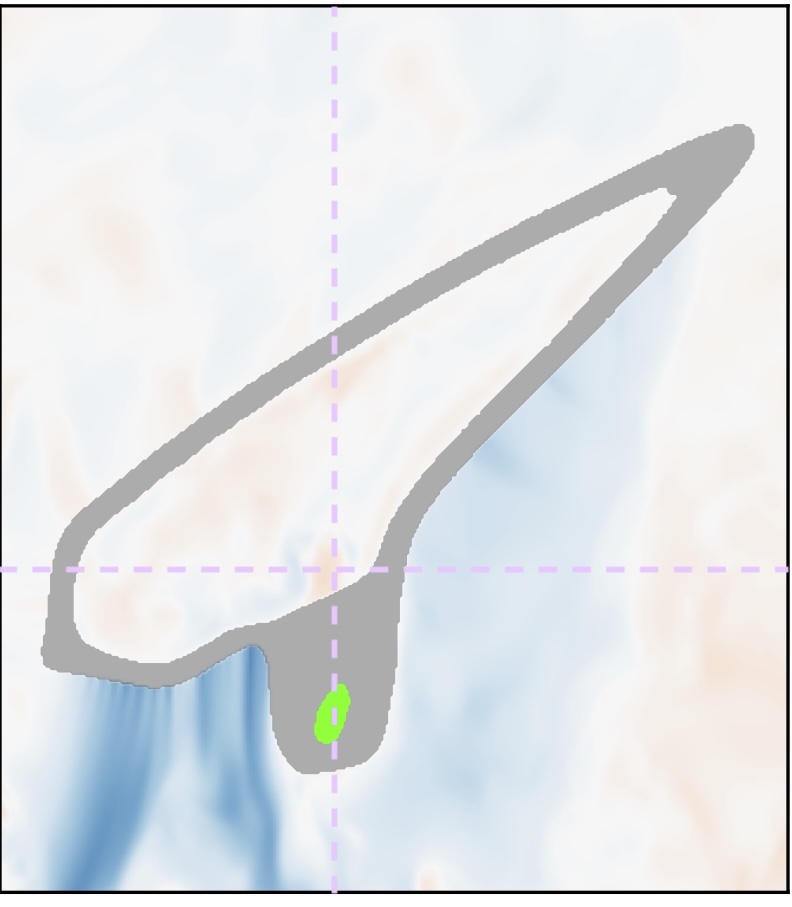
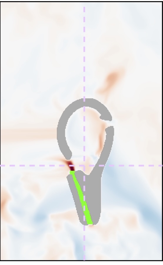
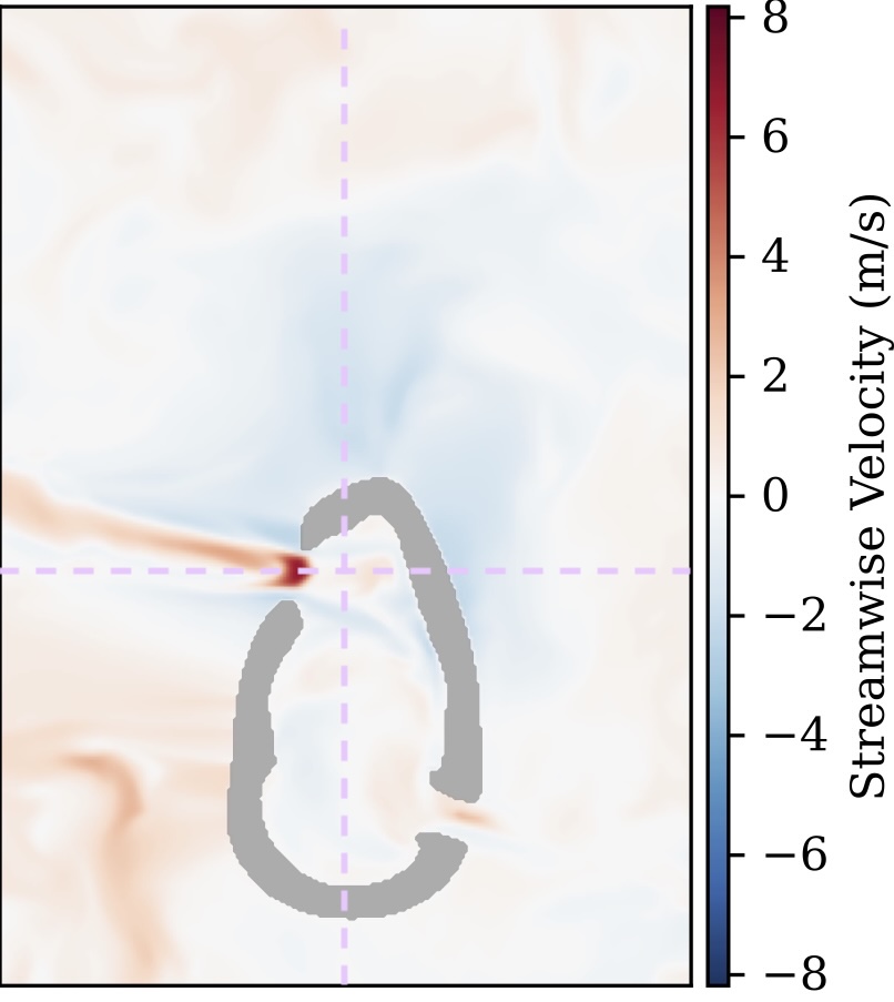
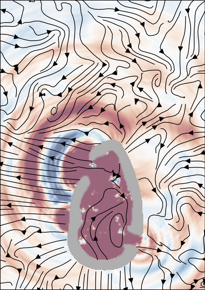
Simulated Results at \(t=0.17\ \mathrm{ms}\)
- Colors: Streamwise Velocity
- Dashed lines: Cut Planes
- Green Region: Inflow
- Colors: Acoustic Pressure
- Arrows: Streamline
Acknowledgments





← Presentation slides
https://jin-woo-lee.github.io/assets/slides/26-isma/slides.html
Web demo →
https://jin-woo-lee.github.io/demos