Numerical Differentiation
Topics in Digital Heritage:
Numerical Methods for Digital Reconstruction
Fall 2026
Why Differentiation? Rates of Change Are Everywhere
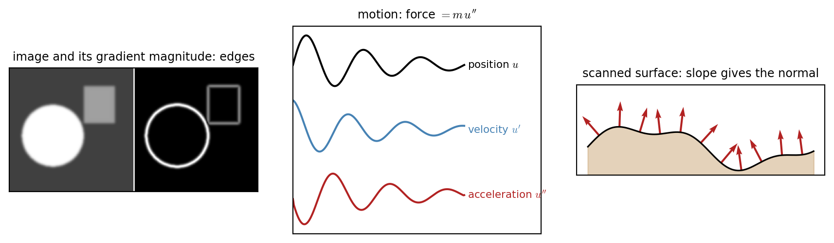
++ gradients and Jacobians for optimization (Newton, Gauss-Newton), physical laws written as differential equations…
Differentiation problem:
given samples \(f(x_1),\dots,f(x_n)\), or a black box that returns \(f(x)\), approximate \(f'(x)\) and \(f''(x)\).
Differentiate the Interpolant
Same idea as quadrature. Write the interpolant in a basis and differentiate the basis:
\[ f(x)\approx\sum_i y_i\,\phi_i(x) \ \Rightarrow\ f'(x)\approx\sum_i y_i\,\phi_i'(x) \]
Piecewise linear “hat” functions have piecewise constant derivatives. On \([x_i, x_{i+1}]\):
\[ f'(x)\approx\frac{y_{i+1}-y_i}{h} \]
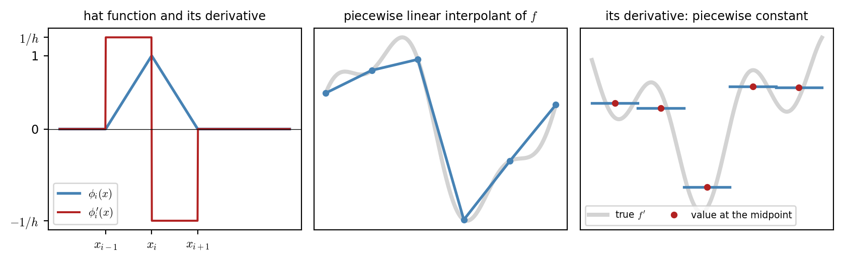
- Differentiation reduces the degree of the interpolant by 1.
- The slope \(\frac{y_{i+1}-y_i}{h}\) matches \(f'\) best at the midpoint of the interval, not at its ends.
- This fact will determine the order of accuracy of finite difference formulas.
Forward, Backward, and Centered Differences
Drop the limit in the definition of the derivative and check with a Taylor series:
\[f(x\pm h) = f(x) \pm h f'(x) + \tfrac{h^2}{2} f''(x) \pm \tfrac{h^3}{6} f'''(x) + \cdots\]
| Formula | Equals | Order | |
|---|---|---|---|
| Forward \(\delta_{+}\) | \(\dfrac{f(x+h)-f(x)}{h}\) | \(f'(x)+\tfrac{h}{2}f''(x)+\cdots\) | \(O(h)\) |
| Backward \(\delta_{-}\) | \(\dfrac{f(x)-f(x-h)}{h}\) | \(f'(x)-\tfrac{h}{2}f''(x)+\cdots\) | \(O(h)\) |
| Centered \(\delta_{\cdot}\) | \(\dfrac{f(x+h)-f(x-h)}{2h}\) | \(f'(x)+\tfrac{h^2}{6}f'''(x)+\cdots\) | \(O(h^2)\) |
def forward(f, x, h):  return (f(x + h) - f(x)) / h
def backward(f, x, h): return (f(x) - f(x - h)) / h
def centered(f, x, h): return (f(x + h) - f(x - h)) / (2 * h)

# when only samples y with spacing h are given
d_fwd = (y[1:] - y[:-1]) / h          # same as np.diff(y) / h
d_ctr = (y[2:] - y[:-2]) / (2 * h)    # interior of np.gradient(y, h)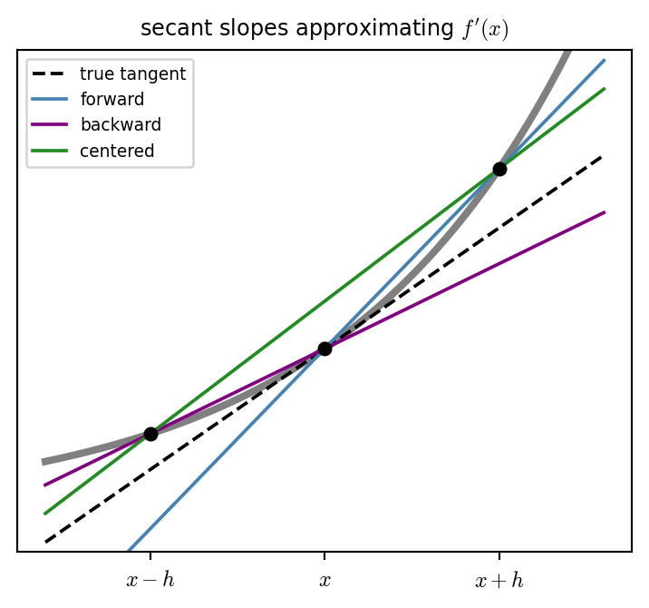
Centered \(=\) average of forward and backward
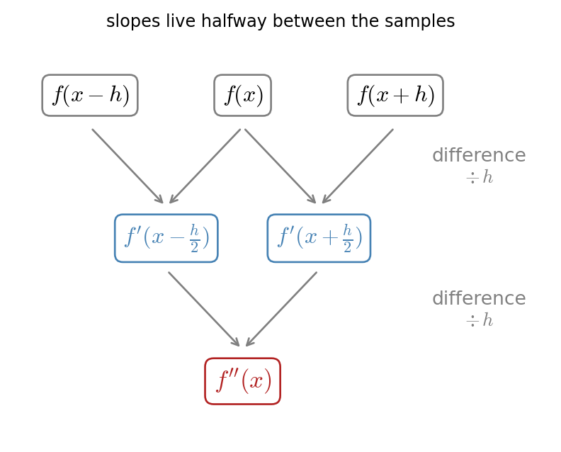
Second Derivative: A Difference of Differences
Add the two Taylor series: odd terms cancel.
\[ f(x+h)+f(x-h) = 2f(x) + h^2 f''(x) + \tfrac{h^4}{12}f''''(x)+\cdots \]
\[ \boxed{\;f''(x) \approx \frac{f(x+h)-2f(x)+f(x-h)}{h^2}\;}\qquad \text{error } O(h^2) \]
Reading 1: a difference of differences, \(\delta_{xx}=\delta_{+}\delta_{-}\)
\[ \frac{1}{h}\left[\frac{f(x+h)-f(x)}{h}-\frac{f(x)-f(x-h)}{h}\right] \]
Reading 2: how far I am from the average of my neighbors
\[ \frac{2}{h^2}\left[\frac{f(x+h)+f(x-h)}{2}-f(x)\right] \]
Measure the Order of Accuracy
Show code
f = lambda x: np.sin(x**2)                                   # test function, differentiated at x0 = 1
df = lambda x: 2 * x * np.cos(x**2)
d2f = lambda x: 2 * np.cos(x**2) - 4 * x**2 * np.sin(x**2)
x0 = 1.0

hs = 2.0 ** -np.arange(1, 11)
rules = [("forward", forward, df(x0), "steelblue"), ("backward", backward, df(x0), "purple"),
         ("centered", centered, df(x0), "forestgreen"), ("second derivative", second, d2f(x0), "firebrick")]

fig, axs = plt.subplots(1, 2, figsize=(9, 3))
for name, rule, exact, col in rules:
    err = np.array([abs(rule(f, x0, h) - exact) for h in hs])
    p = np.polyfit(np.log(hs[3:]), np.log(err[3:]), 1)[0]    # slope in the asymptotic range
    axs[0].loglog(hs, err, "-o", ms=3, color=col, label=f"{name}: slope {p:.2f}")
axs[0].set_xlabel("step size $h$"); axs[0].set_ylabel("|error|")
axs[0].set_title("four formulas, one smooth function", fontsize=9)
axs[0].legend(fontsize=8)

# the same formula on sinusoids of different frequency
for w, col in [(1, "steelblue"), (10, "darkorange"), (100, "firebrick")]:
    s = lambda t: np.sin(w * t)
    rel = np.array([abs(centered(s, x0, h) - w * np.cos(w * x0)) / w for h in hs])
    axs[1].loglog(hs, rel, "-o", ms=3, color=col, label=f"$\\sin({w}\\cdot t)$")
axs[1].set_xlabel("step size $h$"); axs[1].set_ylabel("relative error")
axs[1].set_title("centered difference, three frequencies", fontsize=9)
axs[1].legend(fontsize=8)
plt.tight_layout()
plt.show()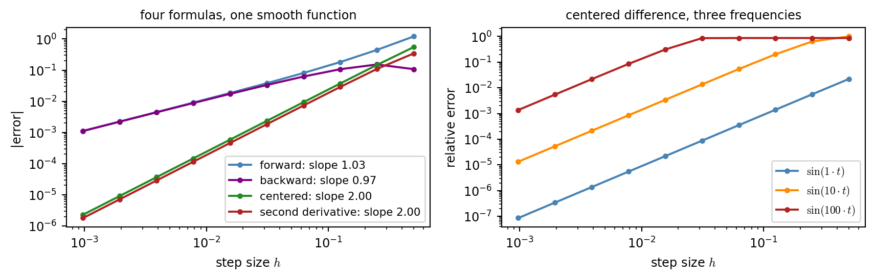
- Forward \(\delta_{+} = f'(x) \color{firebrick}{+ \frac{h}{2} f''(x) + O(h^2)}\)
- Backward \(\delta_{-} = f'(x) \color{firebrick}{- \frac{h}{2} f''(x) + O(h^2)}\)
- Centered \(\delta_{\cdot} = f'(x) \color{firebrick}{+ \frac{h^2}{6} f'''(x) + O(h^4)}\)
- Second derivative \(\delta_{xx} = f''(x) \color{firebrick}{+ \frac{h^2}{12} f''''(x) + O(h^4)}\)
- Errors depend on the derivatives of the function
- Frequency matters: \(\sin(\omega t)\) has \(f''' \sim \omega^3\), \(f'''' \sim \omega^4\)
- On a fixed sampling rate (fixed \(h\)):
- low frequencies are differentiated comparatively well,
- high frequencies are less accurate.
Design Your Own Stencil
Every formula so far is a stencil, a weighted sum of nearby samples: \(f^{(m)}(x)\approx\frac{1}{h^m}\sum_j c_j\,f(x+s_jh)\). Each row is one formula: multiply by the weights, add, scale.
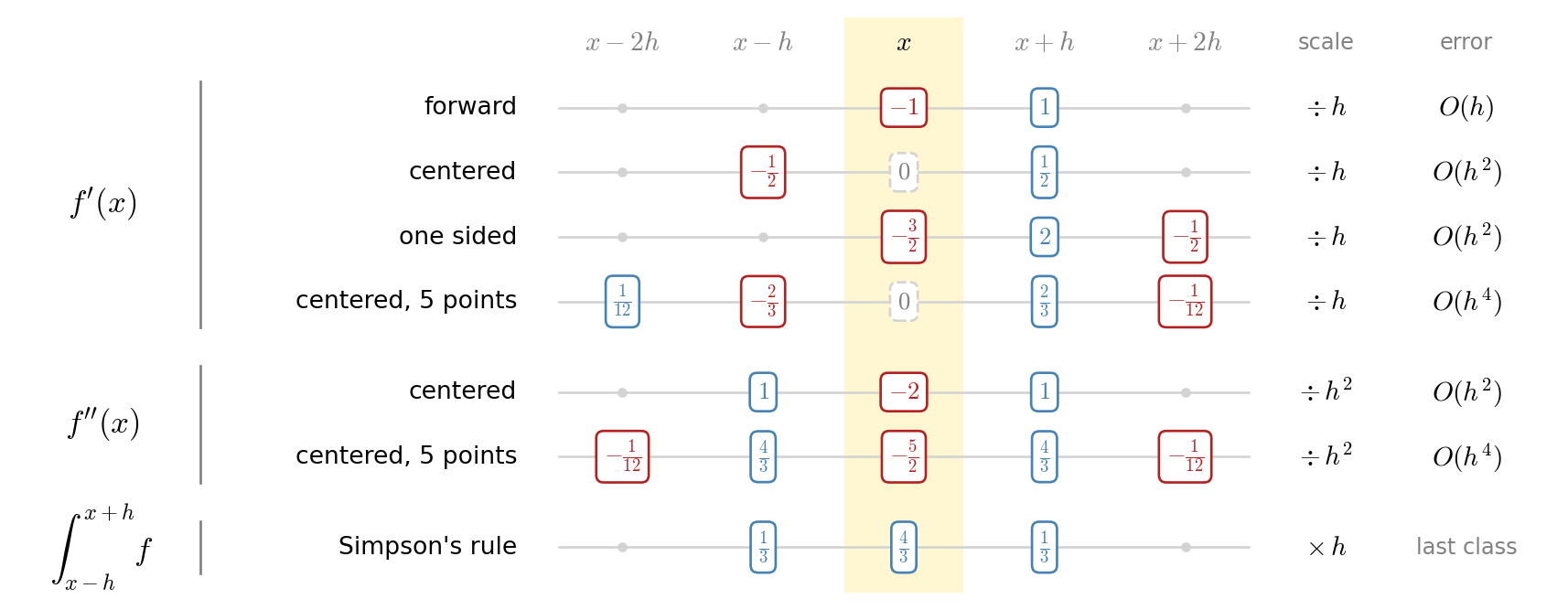
- Derivative weights sum to zero (like constant fn differentiate to zero).
- Wider stencils are more accurate, but harder to use near boundaries and at the first time steps.
- For the ends of a grid where a neighbor is missing, we use one sided stencils (e.g., forward/backward diff).
- Same recipe as Simpson’s rule: fit a parabola through three samples, then integrate it (Simpson) or differentiate it (the three point rows).
- Equivalently: ask for exactness on \(1, t, t^2, \dots\) and solve a small linear system for the weights.
- Symmetry gives a free order in both: Simpson is exact for cubics, centered \(f'\) is \(O(h^2)\).
Richardson Extrapolation
Let \(D(h)\) be the forward difference (1st order accurate) and \(D(h/2)\) the same formula with half the step size. Then
\[ \begin{aligned} D(h) &= f'(x) + \tfrac{h}{2}f''(x) + O(h^2)\\ D(h/2) &= f'(x) + \tfrac{h}{4}f''(x) + O(h^2) \end{aligned} \]
Two equations, two unknowns. Eliminate \(f''\):
\[ 2\,D(h/2) - D(h) = f'(x) + O(h^2) \] Now we have a 2nd order accurate approximation of \(f'(x)\) combining two 1st order approximations.
More generally, if \(D(h)\) is \(p\)-th order accurate, then
gives a \((p+1)\)-th order accurate approximation of \(f'(x)\).
Show code
hs = 2.0 ** -np.arange(1, 9)
curves = [("forward", lambda h: forward(f_test, x0, h), "steelblue", "-"),
          ("Richardson of forward", lambda h: richardson(forward, f_test, x0, h, 1), "steelblue", "--"),
          ("centered", lambda h: centered(f_test, x0, h), "forestgreen", "-"),
          ("Richardson of centered", lambda h: richardson(centered, f_test, x0, h, 2), "forestgreen", "--")]
fig, ax = plt.subplots(figsize=(4.4, 3.9))
for name, D, col, ls in curves:
    err = np.array([abs(D(h) - df_test(x0)) for h in hs])
    p = np.polyfit(np.log(hs[3:]), np.log(err[3:]), 1)[0]
    ax.loglog(hs, err, ls, marker="o", ms=3, color=col, label=f"{name}: slope {p:.1f}")
ax.set_xlabel("step size $h$"); ax.set_ylabel("|error|")
ax.set_title("$f(x)=\\sin x^2$ at $x=1$", fontsize=9)
ax.legend(fontsize=7)
plt.tight_layout()
plt.show()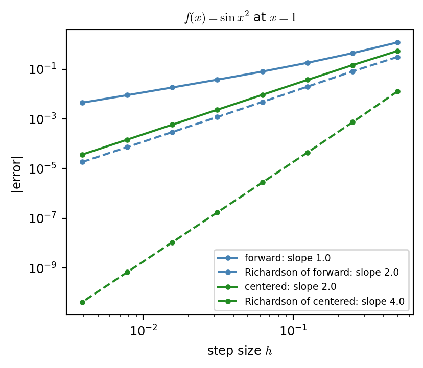
The Catch: You Cannot Take \(h \to 0\)
Why not use \(h=10^{-15}\)?
Cancellation. \(f(x+h)\) and \(f(x)\) agree in almost all digits. Their difference keeps only the rounding error \(\varepsilon\), which is then divided by \(h\):
\[ \lvert\text{error}\rvert \;\lesssim\; \underbrace{\tfrac{h}{2}\lvert f''\rvert}_{\text{truncation}} \;+\; \underbrace{\tfrac{2\varepsilon}{h}}_{\text{rounding}} \]
Smallest at \(h^\star = 2\sqrt{\varepsilon/\lvert f''\rvert}\sim\sqrt{\varepsilon}\).
Example: \(f(x)=\sin x^2\) at \(x=1\)
\(\varepsilon\approx 2.2\cdot 10^{-16}\)
| Formula | Best \(h\) | Best error |
|---|---|---|
| Forward, \(O(h)\) | \(\varepsilon^{1/2}\approx 10^{-8}\) | \(\approx 10^{-8}\) |
| Centered, \(O(h^2)\) | \(\varepsilon^{1/3}\approx 10^{-5}\) | \(\approx 10^{-11}\) |
| Richardson, \(O(h^4)\) | \(\varepsilon^{1/5}\approx 10^{-3}\) | \(\approx 10^{-13}\) |
Higher order reaches an accuracy that no \(h\) can give a lower order formula.
Show code
eps = np.finfo(float).eps
fig, axs = plt.subplots(1, 2, figsize=(5, 2.4))

# truncation: with a large h, the secant is not the tangent
h = 0.3
xs = np.linspace(0.8, 1.45, 200)
axs[0].plot(xs, f_test(xs), color="gray", lw=1, label="$f$")
axs[0].plot(xs, f_test(x0) + df_test(x0) * (xs - x0), "k--", lw=1, label="tangent, $f'(x)$")
axs[0].plot(xs, f_test(x0) + forward(f_test, x0, h) * (xs - x0), color="steelblue", lw=1, label="secant, $D(h)$")
axs[0].plot([x0, x0 + h], f_test(np.array([x0, x0 + h])), "o", ms=4, color="steelblue")
axs[0].set_xticks([x0, x0 + h], ["$x$", "$x+h$"])
axs[0].set_yticks([])
axs[0].set_title("large $h$: truncation", fontsize=9)
axs[0].legend(fontsize=6, loc="lower right")

# rounding: zoom in until one unit is eps, and the computed f is a staircase
h = 2.6 * eps
ts = np.linspace(-1, 7, 801) * eps
stair = lambda t: (f_test(x0 + t) - f_test(x0)) / eps          # computed values, in units of eps
axs[1].plot(ts / eps, stair(ts), color="gray", lw=1, label="computed $f$")
axs[1].plot(ts / eps, df_test(x0) * ts / eps, "k--", lw=1, label="tangent, $f'(x)$")
axs[1].plot(ts / eps, forward(f_test, x0, h) * ts / eps, color="firebrick", lw=1, label="secant, $D(h)$")
axs[1].plot([0, h / eps], [0, stair(h)], "o", ms=4, color="firebrick")
axs[1].set_xticks([0, h / eps], ["$x$", "$x+h$"])
axs[1].set_ylim(-1.5, 9.5)
axs[1].set_ylabel("$(f - f(x))\\,/\\,\\varepsilon$", fontsize=7)
axs[1].set_title(f"tiny $h={h / eps:.1f}\\,\\varepsilon$: rounding", fontsize=9)
axs[1].legend(fontsize=6, loc="upper left")
plt.tight_layout()
plt.show()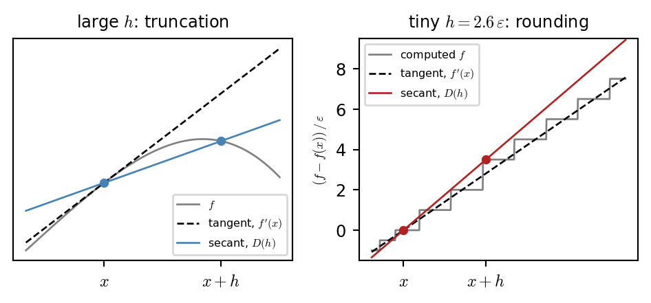
Show code
eps = np.finfo(float).eps
hs = np.logspace(-16, 0, 400)
curves = [("forward", lambda h: forward(f_test, x0, h), "steelblue", eps ** (1 / 2)),
          ("centered", lambda h: centered(f_test, x0, h), "forestgreen", eps ** (1 / 3)),
          ("Richardson of centered", lambda h: richardson(centered, f_test, x0, h, 2), "firebrick", eps ** (1 / 5))]
fig, ax = plt.subplots(figsize=(5, 2.4))
for name, D, col, h_best in curves:
    err = np.array([abs(D(h) - df_test(x0)) for h in hs])
    ax.loglog(hs, np.maximum(err, 1e-17), color=col, lw=1, label=name)
    ax.axvline(h_best, color=col, ls=":", lw=1)                 # predicted best step size
ax.loglog(hs, eps / hs, color="k", ls="--", lw=1, label="rounding: $\\varepsilon/h$")
ax.set_ylim(1e-15, 10)
ax.set_xlabel("step size $h$"); ax.set_ylabel("|error|")
ax.set_title("truncation error (right) against rounding error (left)", fontsize=9)
ax.legend(fontsize=7, loc="lower left")
plt.tight_layout()
plt.show()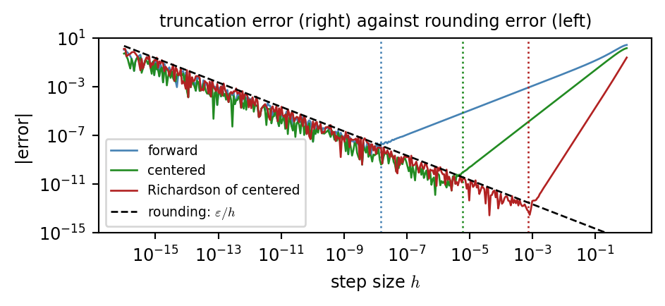
Measured Data: Noise Sets the Step Size
Show code
fs = 100.0                                    # samples per second
h = 1 / fs
t = np.arange(0, 2, h)
u = lambda t: np.sin(2 * np.pi * 1.0 * t) + 0.3 * np.sin(2 * np.pi * 2.3 * t)
du = lambda t: 2 * np.pi * 1.0 * np.cos(2 * np.pi * 1.0 * t) + 0.3 * 2 * np.pi * 2.3 * np.cos(2 * np.pi * 2.3 * t)
y = u(t) + 0.02 * rng.standard_normal(t.size)                   # measured position

def wide_centered(y, m, h):                   # centered difference with step m * h
    return (y[2 * m:] - y[:-2 * m]) / (2 * m * h)

rms = lambda est, tt: np.sqrt(np.mean((est - du(tt)) ** 2))
strides = np.arange(1, 21)
errs = [rms(wide_centered(y, m, h), t[m:-m]) for m in strides]
sg = savgol_filter(y, window_length=21, polyorder=3, deriv=1, delta=h)   # fit a local cubic, differentiate it
inner = slice(10, -10)

fig, axs = plt.subplots(1, 3, figsize=(9, 3.3), width_ratios=[1, 1.3, 1])
axs[0].plot(t, y, ".", color="firebrick", ms=3, label="measured")
axs[0].plot(t, u(t), color="k", lw=1, label="true")
axs[0].set_title("position samples, 2% noise", fontsize=9); axs[0].set_xlabel("$t$ (s)")
axs[0].legend(fontsize=7, loc="lower left"); axs[0].set_ylim(-2.1, 1.3)

axs[1].plot(t[:-1], np.diff(y) / h, color="silver", lw=0.8, label="np.diff(y) / h")
axs[1].plot(t[4:-4], wide_centered(y, 4, h), color="steelblue", lw=1.3, label="centered, step $4h$")
axs[1].plot(t[inner], sg[inner], color="darkorange", lw=1.3, label="smooth, then differentiate")
axs[1].plot(t, du(t), color="k", lw=1, label="true velocity")
axs[1].set_title("estimated velocity", fontsize=9); axs[1].set_xlabel("$t$ (s)")
axs[1].legend(fontsize=6, ncol=2, loc="upper center", handlelength=1.2, columnspacing=0.8)
axs[1].set_ylim(-15, 26)

axs[2].semilogy(strides, errs, "-o", ms=3, color="steelblue", label="centered, step $mh$")
axs[2].axhline(rms(sg[inner], t[inner]), color="darkorange", ls="--", label="smooth, then differentiate")
axs[2].set_xlabel("step in samples $m$"); axs[2].set_ylabel("RMS error of velocity")
axs[2].set_xticks([1, 5, 10, 15, 20])
axs[2].set_title("noise (left) against truncation (right)", fontsize=9)
axs[2].set_ylim(0.15, 12)
axs[2].legend(fontsize=7, loc="upper center")
plt.tight_layout()
plt.show()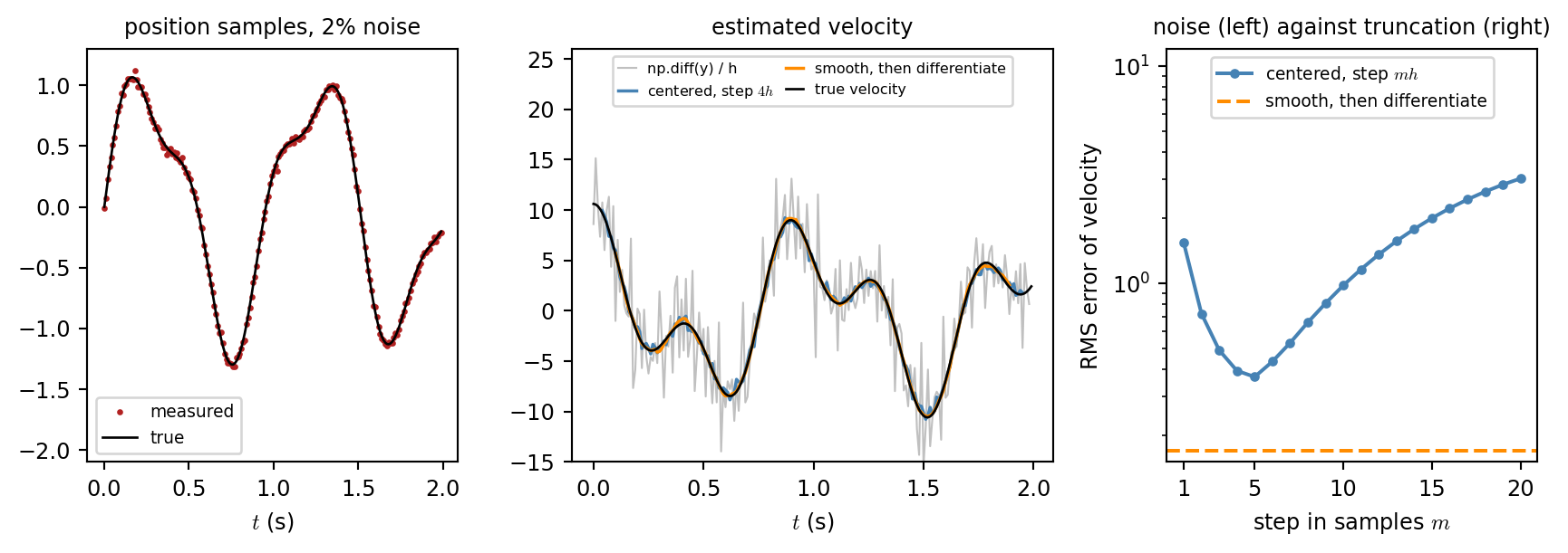
Same bound with \(\varepsilon\) = sensor noise: \(\ \lvert\text{error}\rvert\lesssim \tfrac{2\varepsilon}{h}+O(h)\). Here a larger step gives a better derivative.
Better still: fit a smooth local model (least squares), then differentiate the model.
Difference Operators Are Filters
Feed in one sinusoid \(u(t)=e^{j\omega t}\), then the derivative multiplies it by \(j\omega\). Same for sampled version \(u^n = e^{j\omega k n}\) and the finite difference \(\delta_t\).
| Operator | Multiplies \(u\) by |
|---|---|
| \(\dfrac{d}{dt}\) | \(j\omega\) |
| \(\delta_{t+}\) | \(\dfrac{e^{j\omega k}-1}{k}\), size \(\dfrac{2}{k}\left\lvert\sin\dfrac{\omega k}{2}\right\rvert\) |
| \(\delta_{t\cdot}\) | \(\dfrac{j\sin\omega k}{k}\) |
| \(\delta_{tt}\) | \(-\dfrac{4}{k^2}\sin^2\dfrac{\omega k}{2}\) |
Show code
th = np.linspace(0, np.pi, 300)                        # theta = omega * k, from 0 to Nyquist
fig, axs = plt.subplots(1, 2, figsize=(5.6, 4.2))
axs[0].plot(th, th, "k--", lw=1, label="exact: $\\omega k$")
axs[0].plot(th, np.abs(np.exp(1j * th) - 1), color="steelblue", label="forward / backward")
axs[0].plot(th, np.abs(np.sin(th)), color="forestgreen", label="centered")
axs[0].set_title("first derivative: gain $\\times\\,k$", fontsize=9)
axs[1].plot(th, th**2, "k--", lw=1, label="exact: $(\\omega k)^2$")
axs[1].plot(th, 4 * np.sin(th / 2) ** 2, color="firebrick", label="second difference")
axs[1].set_title("second derivative: gain $\\times\\,k^2$", fontsize=9)
for ax in axs:
    ax.set_xticks([0, np.pi / 4, np.pi / 2, np.pi])
    ax.set_xticklabels(["0", "$\\pi/4$", "$\\pi/2$", "$\\pi$"])
    ax.set_xlabel("frequency $\\omega k$  ($\\pi$ = Nyquist)")
    ax.legend(fontsize=7, loc="upper left")
plt.tight_layout()
plt.show()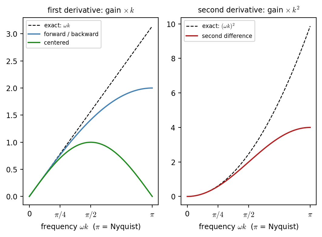
- Low frequency: all agree with \(j\omega\). Accuracy means many samples per period.
- Gain grows with frequency: noise lives at high frequency, so it is amplified most.
- Centered is blind at Nyquist: \(+1,-1,+1,\dots\) has centered difference \(0\).
Differentiation Is a Matrix
Stack the samples in a vector \(\mathbf{u}\). Each row of the matrix is one stencil:
\[ \mathbf{D}_{xx}\mathbf{u}=\frac{1}{h^2} \begin{bmatrix} -2 & 1 & & \\ 1 & -2 & 1 & \\ & \ddots & \ddots & \ddots \\ & & 1 & -2 \end{bmatrix} \begin{bmatrix}u_1\\u_2\\\vdots\\u_n\end{bmatrix} \]
Show code
def D_xx(n, h):
    return sp.diags([1, -2, 1], [-1, 0, 1], shape=(n, n)) / h**2

fig, axs = plt.subplots(2, 1, figsize=(3.5, 3.5), height_ratios=[1.25, 1])
A = (D_xx(7, 1.0)).toarray()                           # the pattern, in units of 1 / h^2
axs[0].imshow(A, cmap="RdBu", vmin=-4, vmax=4)
for (i, j), v in np.ndenumerate(A):
    if v != 0:
        axs[0].text(j, i, f"{v:.0f}", ha="center", va="center", fontsize=8)
axs[0].set_xticks([]); axs[0].set_yticks([])
axs[0].set_title("$h^2\\,\\mathbf{D}_{xx}$ for $n=7$: tridiagonal", fontsize=9)

n = 15                                                 # interior points of [0, 1], u = 0 at both ends
h = 1 / (n + 1)
x = h * np.arange(1, n + 1)
xs = np.linspace(0, 1, 200)
axs[1].plot(xs, -np.pi**2 * np.sin(np.pi * xs), color="lightgray", lw=3, label="exact $u''$")
axs[1].plot(x, D_xx(n, h) @ np.sin(np.pi * x), "o", color="firebrick", ms=4, label="$\\mathbf{D}_{xx}\\mathbf{u}$")
axs[1].plot(x, np.sin(np.pi * x), "-o", color="steelblue", ms=3, lw=1, label="$u=\\sin\\pi x$")
axs[1].legend(fontsize=7, ncol=3, loc="lower center")
axs[1].set_ylim(-14, 2); axs[1].set_xlabel("$x$")
plt.tight_layout()
plt.show()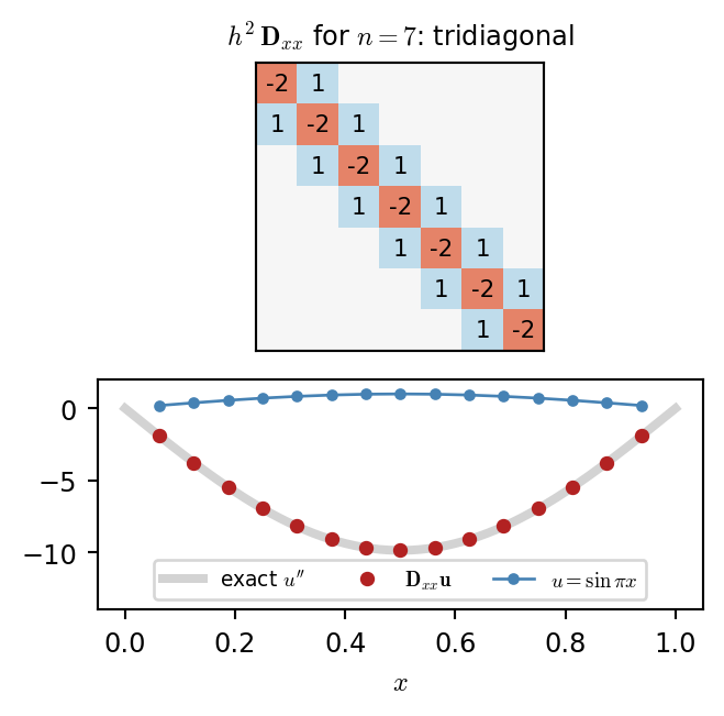
- First and last rows are cut off: this assumes \(u=0\) outside (fixed ends). Otherwise use a one sided stencil there.
- Reverse direction: solving \(u''=g\) becomes the sparse linear system \(\mathbf{D}_{xx}\mathbf{u}=\mathbf{g}\) (the Poisson system from the iterative solvers class).
Images: Gradient and Laplacian
One axis at a time, exactly like bilinear interpolation and iterated quadrature. Each formula is a small stencil slid over the pixel grid:
\[ \frac{\partial f}{\partial x}\approx\frac{f_{i,j+1}-f_{i,j-1}}{2h} \;\;\Leftrightarrow\;\; \tfrac{1}{2h}\begin{bmatrix}-1&0&1\end{bmatrix} \qquad \nabla^2 f\approx\frac{f_{i+1,j}+f_{i-1,j}+f_{i,j+1}+f_{i,j-1}-4f_{i,j}}{h^2} \;\;\Leftrightarrow\;\; \tfrac{1}{h^2}\begin{bmatrix}&1&\\1&-4&1\\&1&\end{bmatrix} \]
Show code
u = np.linspace(-1, 1, 200)
U, V = np.meshgrid(u, u)
img = 0.2 + 0.6 * ((U + 0.3)**2 + (V - 0.1)**2 < 0.25) + 0.3 * ((np.abs(U - 0.45) < 0.25) & (np.abs(V + 0.4) < 0.3))
img = gaussian_filter(img, 2) + 0.004 * rng.standard_normal(img.shape)       # a soft image with a little sensor noise

fx = np.zeros_like(img); fy = np.zeros_like(img); lap = np.zeros_like(img)
fx[:, 1:-1] = (img[:, 2:] - img[:, :-2]) / 2                                 # centered difference along x (h = 1 pixel)
fy[1:-1, :] = (img[2:, :] - img[:-2, :]) / 2                                 # centered difference along y
lap[1:-1, 1:-1] = (img[2:, 1:-1] + img[:-2, 1:-1] + img[1:-1, 2:] + img[1:-1, :-2] - 4 * img[1:-1, 1:-1])

fig, axs = plt.subplots(1, 4, figsize=(9, 2.6))
panels = [(img, "image $f$", "gray", None), (fx, "$\\partial f/\\partial x$", "RdBu_r", np.abs(fx).max()),
          (np.hypot(fx, fy), "$\\|\\nabla f\\|$: edges", "gray", None), (lap, "Laplacian $\\nabla^2 f$", "RdBu_r", np.abs(lap).max())]
for ax, (im, ttl, cmap, lim) in zip(axs, panels):
    ax.imshow(im, cmap=cmap, vmin=None if lim is None else -lim, vmax=lim)
    ax.set_title(ttl, fontsize=9); ax.set_xticks([]); ax.set_yticks([])
plt.tight_layout()
plt.show()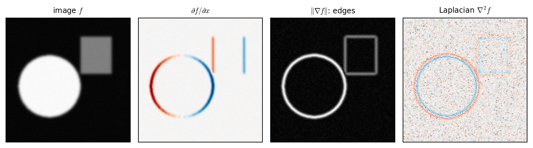
The Laplacian is much noisier: second differences amplify high frequencies by \(\omega^2\).
Sometimes we combine differentiation and smoothing, e.g.,
- Sobel filter: \(\tfrac{1}{8h}\left[\begin{smallmatrix}-1&0&1\\-2&0&2\\-1&0&1\end{smallmatrix}\right]\) = difference along \(x\) times average \([1,2,1]\) along \(y\).
Application: Relighting a Domed Medallion Scan
- Goal: Given a scanned height map \(z(x,y)\) relight it from any light direction \(\boldsymbol{\ell}\).
- Brightness depends on the surface normal, which is a derivative of the height (denoting \(z_x=\partial z/\partial x\), \(z_y=\partial z/\partial y\)):
\[ \mathbf{n}=\frac{(-z_x,\,-z_y,\,1)}{\sqrt{z_x^2+z_y^2+1}},\qquad \text{brightness}=\max(0,\ \mathbf{n}\cdot\boldsymbol{\ell})\quad\text{for a light direction }\boldsymbol{\ell}. \]
Show code
from matplotlib.textpath import TextPath

# synthetic "scan": a domed medallion with a rim and a shallow raised inscription
n = 260
h = 2 / (n - 1)                                        # grid spacing
X, Y = np.meshgrid(np.linspace(-1, 1, n), np.linspace(1, -1, n))
R = np.hypot(X, Y)
text = TextPath((0, 0), "KAIST", size=1)
lo, hi = text.vertices.min(0), text.vertices.max(0)
scale = (hi[0] - lo[0]) / 1.3                          # make the text 1.3 units wide
pts = np.stack([X.ravel() * scale + 0.5 * (lo[0] + hi[0]), Y.ravel() * scale + 0.5 * (lo[1] + hi[1])], 1)
letters = text.contains_points(pts).reshape(n, n).astype(float)
ring = (np.abs(R - 0.86) < 0.035).astype(float)
z = 0.15 * np.sqrt(np.clip(1 - (R / 1.05)**2, 0, None)) + 0.012 * gaussian_filter(letters + ring, 2.0)
z[R > 0.95] = 0

# normals from finite differences of the height
z_y, z_x = np.gradient(z, -h, h)                       # rows run along -y, columns along +x
N = np.stack([-z_x, -z_y, np.ones_like(z)], -1) / np.sqrt(z_x**2 + z_y**2 + 1)[..., None]

def shade(N, azimuth, elevation):                      # Lambertian shading for a distant light
    a, e = np.radians(azimuth), np.radians(elevation)
    return np.clip(N @ np.array([np.cos(e) * np.cos(a), np.cos(e) * np.sin(a), np.sin(e)]), 0, 1)

fig, axs = plt.subplots(1, 4, figsize=(9, 2.7))
axs[0].imshow(z, cmap="gray"); axs[0].set_title("height map $z(x,y)$", fontsize=9)
axs[1].imshow((0.5 * (N * [2.5, 2.5, 1] + 1)).clip(0, 1)); axs[1].set_title("normal map (from $z_x, z_y$)", fontsize=9)
axs[2].imshow(shade(N, 180, 20), cmap="gray", vmin=0); axs[2].set_title("raking light from the left", fontsize=9)
axs[3].imshow(shade(N, 90, 20), cmap="gray", vmin=0); axs[3].set_title("raking light from the top", fontsize=9)
for ax in axs:
    ax.set_xticks([]); ax.set_yticks([])
plt.tight_layout()
plt.show()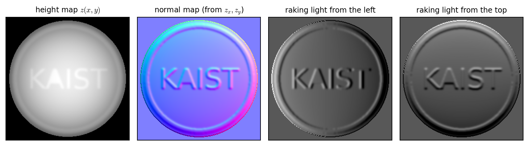
cf. Real scans are noisy, and differentiation amplifies that noise: smooth first, or use a wider stencil.
Simple Harmonic Oscillation (SHO)
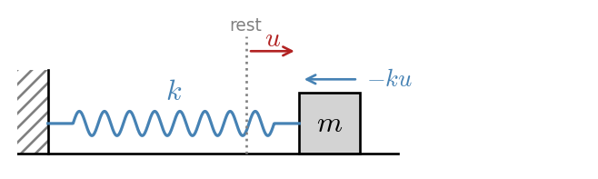
A mass on a spring is the building block of most vibrating instruments.
Recall Hooke’s law: the spring pulls back with its constant \(k\).
\[ m\frac{d^2 u}{dt^2}=-ku \qquad \Rightarrow \qquad \frac{d^2 u}{dt^2}+\omega_0^2\,u=0,\quad \omega_0=\sqrt{k/m} \]
The analytic solution is \(u(t)=\cos\omega_0 t\). Yet, we can also solve it numerically.
Replace \(\tfrac{d^2}{dt^2}\) by the finite difference operator \(\delta_{tt}\) with time step \(k=1/f_s\):
\[ \frac{u^{n+1}-2u^n+u^{n-1}}{k^2} + \omega_0^2\,u^n = 0 \ \ \Rightarrow\ \ \boxed{u^{n+1}=(2-\omega_0^2k^2)\,u^n-u^{n-1}} \]
How does it behave?
To analyze the scheme, insert ansatz \(u^n = e^{j\omega n k}\) to the recurrence above:
\[\begin{aligned} e^{j\omega (n+1) k}=(2-\omega_0^2k^2)e^{j\omega n k}-e^{j\omega (n-1) k}\quad&\Rightarrow\quad e^{j\omega k}=(2-\omega_0^2k^2)-e^{-j\omega k} \\ &\Rightarrow\quad 2\cos(\omega k)=2-\omega_0^2k^2 \\ &\Rightarrow\quad \frac{2}{k}\sin\frac{\omega k}{2}=\omega_0 \end{aligned}\]
Remark. Numerical Dispersion
- The output oscillates at \(\omega\) with \(\tfrac{2}{k}\sin\tfrac{\omega k}{2}=\omega_0\).
- If \(k\to0\), then \(\omega\to\omega_0\) (the scheme is consistent).
- For \(k>0\), \(\omega>\omega_0\) (numerical dispersion).
- \(\sin(\cdot) \leq 1\ \Rightarrow\ \omega_0 \leq \tfrac{2}{k}\)
- Stable only if \(\omega_0 k \leq 2\ \) (equiv. \((2\pi f_0)/f_s \leq 2\))
- That is \(f_0\leq f_s/\pi\)
(stricter than the Nyquist limit)
SHO Results
Show code
def simple_harmonic_oscillator(f0, fs, n_steps, u0=1.0):
    a = 2 * np.pi * f0 / fs                             # omega_0 * k
    u = np.zeros(n_steps)
    u[0], u[1] = u0, u0 * (1 - a**2 / 2)
    for n in range(1, n_steps - 1):
        u[n + 1] = (2 - a**2) * u[n] - u[n - 1]
    return u

fig, axs = plt.subplots(1, 3, figsize=(10, 2.5))

f0, fs, n = 1000.0, 8000.0, 41                          # accuracy: 8 samples per period
tt = np.linspace(0, (n - 1) / fs, 1000)
f_num = fs / np.pi * np.arcsin(np.pi * f0 / fs)         # frequency of the numerical solution
axs[0].plot(1e3 * tt, np.cos(2 * np.pi * f0 * tt), color="lightgray", lw=3, label="exact, 1000 Hz")
axs[0].plot(1e3 * np.arange(n) / fs, simple_harmonic_oscillator(f0, fs, n), "-o", color="steelblue", ms=3, lw=1, label=f"scheme, {f_num:.0f} Hz")
axs[0].set_xlabel("time (ms)"); axs[0].set_ylim(-1.7, 1.3)
axs[0].set_title("$f_s=8$ kHz: right amplitude, sharp pitch", fontsize=9)
axs[0].legend(fontsize=7, loc="lower left", ncol=2)

for fs_, col in [(44100.0, "steelblue"), (96000.0, "forestgreen")]:      # pitch error in cents
    f = np.geomspace(50, 10000, 200)
    cents = 1200 * np.log2(fs_ / np.pi * np.arcsin(np.pi * f / fs_) / f)
    axs[1].semilogx(f, cents, color=col, label=f"$f_s$ = {fs_ / 1000:g} kHz")
axs[1].axhline(5, color="gray", ls=":", lw=1); axs[1].text(55, 7, "about audible (5 cents)", fontsize=7, color="gray")
axs[1].set_xlabel("$f_0$ (Hz)"); axs[1].set_ylabel("pitch error (cents)"); axs[1].set_ylim(0, 60)
axs[1].set_title("frequency warping", fontsize=9)
axs[1].legend(fontsize=7)

u_bad = simple_harmonic_oscillator(2600.0, 8000.0, 60)                  # stability: omega_0 k = 2.04 > 2
axs[2].semilogy(np.abs(u_bad), "-o", color="firebrick", ms=3, lw=1)
axs[2].set_xlabel("time step $n$"); axs[2].set_ylabel("$|u^n|$")
axs[2].set_title("$f_0=2.6$ kHz: $\\omega_0k>2$, unstable", fontsize=9)
plt.tight_layout()
plt.show()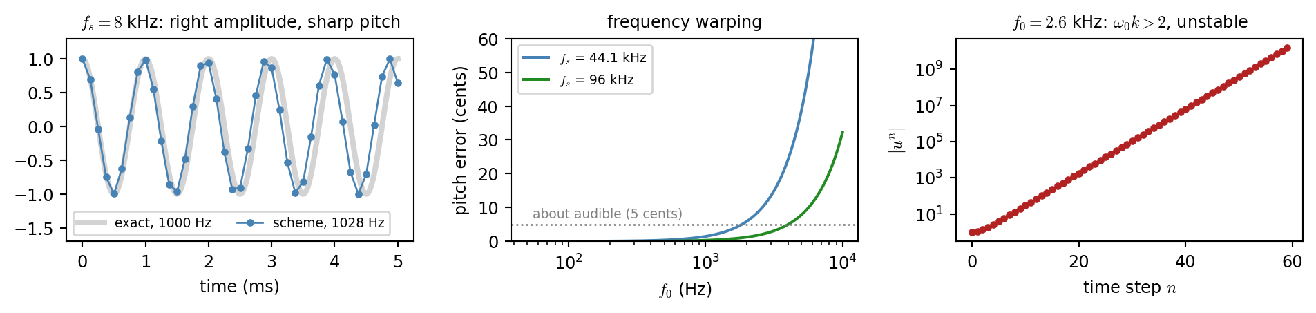
Energy Analysis: The Scheme
Repeat the same steps on the scheme \(\delta_{tt}u+\omega_0^2u=0\). Multiply it by \(\delta_{t\cdot}u\), to get \((\delta_{t\cdot}u)\,\delta_{tt}u+\omega_0^2\,(\delta_{t\cdot}u)\,u=0\).
Then use two identities below (cf. Bilbao Section 2.2.4)
\[ (\delta_{t\cdot}u)(\delta_{tt}u)=\delta_{t+}\Big[\tfrac{1}{2}(\delta_{t-}u)^2\Big] \quad\text{and}\quad (\delta_{t\cdot}u)\,u=\delta_{t+}\Big[\tfrac{1}{2}u^nu^{n-1}\Big] \]
to acquire
\[\begin{aligned} \delta_{t+}\Big[\underbrace{\tfrac{1}{2}(\delta_{t-}u)^2}_{\mathfrak{t}^n}+\underbrace{\tfrac{\omega_0^2}{2}u^nu^{n-1}}_{\mathfrak{v}^n}\Big]=0 \quad\Rightarrow\quad \delta_{t+}\mathfrak{h}^n=0\quad (\mathfrak{h}^n=\mathfrak{t}^n+\mathfrak{v}^n) \end{aligned}\]
so the scheme conserves energy \(\mathfrak{h}^n\) exactly and for any \(k\):
\[ \boxed{\mathfrak{h}^{n+1}=\mathfrak{h}^n,\qquad \mathfrak{t}^n=\tfrac{1}{2}\Big(\frac{u^n-u^{n-1}}{k}\Big)^2,\qquad \mathfrak{v}^n=\tfrac{\omega_0^2}{2}\,u^n\,u^{n-1}} \]
Is the scheme always stable, then?
No. \(\mathfrak{v}^n\) is a product of two different samples, so it can be negative.
\[\begin{aligned} \mathfrak{h}^n=\frac{1}{2k^2}\Big[(u^n)^2+(u^{n-1})^2-(2-\omega_0^2k^2)\,u^n\,u^{n-1}\Big] \end{aligned}\]
This quadratic form is positive definite only if \(\lvert 2-\omega_0^2k^2\rvert<2\), that is \(\omega_0k<2\): the same stability condition, found without any sinusoid.
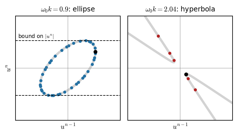
Each dot is a pair \((u^{n-1},u^n)\).
Conservation keeps all of them on one level set of \(\mathfrak{h}\).
Remark. Stability from Energy
- \(\omega_0k<2\): the level set is an ellipse. It is closed, so
\(\lvert u^n\rvert\leq\sqrt{\dfrac{2k^2\,\mathfrak{h}^1}{1-(1-\omega_0^2k^2/2)^2}}\) - \(\omega_0k>2\): the level set is a hyperbola. The energy is still conserved, but the dots run away along it.
- \(\mathfrak{h}^n\) uses \(u^n\) and \(u^{n-1}\): it lives at the half step \(t=(n-\tfrac{1}{2})k\).
Energy Analysis Results
Show code
def scheme(w0, k, u0, u1, n_steps):
    u = np.zeros(n_steps)
    u[0], u[1] = u0, u1
    for n in range(1, n_steps - 1):
        u[n + 1] = (2 - w0**2 * k**2) * u[n] - u[n - 1]
    return u

def discrete_energy(u, k, w0):                          # entry n-1 holds the energy at time (n - 1/2) k
    kinetic = 0.5 * ((u[1:] - u[:-1]) / k) ** 2
    potential = 0.5 * w0**2 * u[1:] * u[:-1]
    return kinetic, potential

fig, axs = plt.subplots(1, 3, figsize=(10, 2.5))

w0, k = 1.0, 0.1                                        # stable: omega_0 k = 0.1
u = scheme(w0, k, 0.2, -0.4, 62)
kin, pot = discrete_energy(u, k, w0)
h_tot = kin + pot
n = np.arange(1, u.size)
axs[0].plot(n, kin, color="firebrick", lw=1.2, label="kinetic $\\mathfrak{t}^n$")
axs[0].plot(n, pot, color="steelblue", lw=1.2, label="potential $\\mathfrak{v}^n$")
axs[0].plot(n, h_tot, color="k", lw=1.8, label="total $\\mathfrak{h}^n$")
axs[0].set_xlabel("time step $n$"); axs[0].set_ylim(-1, 25)
axs[0].set_title("$\\omega_0k=0.1$: energy is traded, the total stays", fontsize=9)
axs[0].legend(fontsize=7, ncol=3, loc="upper center", handlelength=1.2, columnspacing=0.8)

eps = np.finfo(float).eps                               # relative change of the total, in units of eps
axs[1].plot(n, (h_tot - h_tot[0]) / h_tot[0] / eps, ".", color="k", ms=4)
axs[1].set_xlabel("time step $n$")
axs[1].set_ylabel("$(\\mathfrak{h}^n-\\mathfrak{h}^1)\\,/\\,\\mathfrak{h}^1$, in units of $\\varepsilon$")
axs[1].grid(axis="y", color="lightgray", lw=0.6)
axs[1].set_title("conserved to machine precision", fontsize=9)

w0, k = 2 * np.pi * 2600.0, 1 / 8000.0                  # unstable: omega_0 k = 2.04 > 2
u = scheme(w0, k, 1.0, 1 - (w0 * k)**2 / 2, 26)
kin, pot = discrete_energy(u, k, w0)
h_tot = kin + pot
n = np.arange(1, u.size)
axs[2].semilogy(n, kin / abs(h_tot[0]), "-o", color="firebrick", ms=3, lw=1, label="$\\mathfrak{t}^n$")
axs[2].semilogy(n, -pot / abs(h_tot[0]), "-o", color="steelblue", ms=2, lw=1, label="$-\\mathfrak{v}^n$")
axs[2].semilogy(n, np.abs(h_tot) / abs(h_tot[0]), color="k", lw=1.8, label="$|\\mathfrak{h}^n|$")
axs[2].set_xlabel("time step $n$"); axs[2].set_ylabel("energy / $|\\mathfrak{h}^1|$")
axs[2].set_title("$\\omega_0k=2.04$: still conserved, but $\\mathfrak{v}^n<0$", fontsize=9)
axs[2].legend(fontsize=7, loc="upper left")
plt.tight_layout()
plt.show()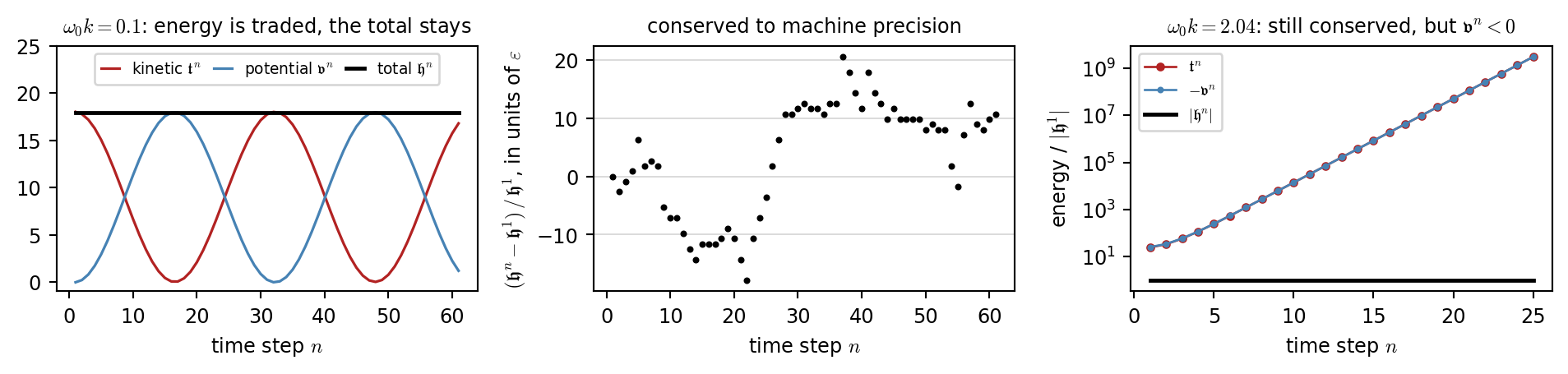
- Stable case: \(\mathfrak{t}^n\) and \(\mathfrak{v}^n\) trade places, and their sum is flat.
- The only change left is rounding
- a few tens of \(\varepsilon\approx2.2\cdot10^{-16}\).
- A free debugging tool: plot the energy of your simulation. A drift far above \(\varepsilon\) means a bug.
- Unstable case: \(\mathfrak{h}^n\) is still constant, but it is a huge positive \(\mathfrak{t}^n\) plus a huge negative \(\mathfrak{v}^n\).
- Conservation alone bounds nothing.
- Stability \(=\) conserved and positive definite.
Stability and Damping of Euler Methods
We may split \(u''=-\omega_0^2u\) into two first-order equations, with the scaled velocity \(w=u'/\omega_0\):
\[ u'=\omega_0\,w,\qquad w'=-\omega_0\,u \]
Then pick a first difference for each equation. With \(a=\omega_0k\):
| one step | eliminate \(w\) | |
|---|---|---|
| Forward Euler \(\delta_{t+}\) for both |
\(u^{n+1}=u^n+a\,w^n\) \(w^{n+1}=w^n-a\,u^n\) |
\(\delta_{tt}u^n=-\omega_0^2\,u^{\color{firebrick}{n-1}}\) |
| Backward Euler \(\delta_{t-}\) for both |
\(u^{n+1}=u^n+a\,w^{n+1}\) \(w^{n+1}=w^n-a\,u^{n+1}\) |
\(\delta_{tt}u^n=-\omega_0^2\,u^{\color{firebrick}{n+1}}\) |
| One of each \(\delta_{t+}\) for \(u\), \(\delta_{t-}\) for \(w\) |
\(u^{n+1}=u^n+a\,w^n\) \(w^{n+1}=w^n-a\,u^{n+1}\) |
\(\delta_{tt}u^n=-\omega_0^2\,u^{n}\) |
All three have the same \(\delta_{tt}\). They differ in when the spring force is evaluated.
Why does one grow and the other decay?
Try \(u^n=z^n\). The amplitude is multiplied by \(|z|\) every step:
\[ \color{#c0392b}{z=1\pm ja,\ \ |z|=\sqrt{1+a^2}>1} \qquad \color{#8e44ad}{z=\frac{1}{1\mp ja},\ \ |z|=\frac{1}{\sqrt{1+a^2}}<1} \]
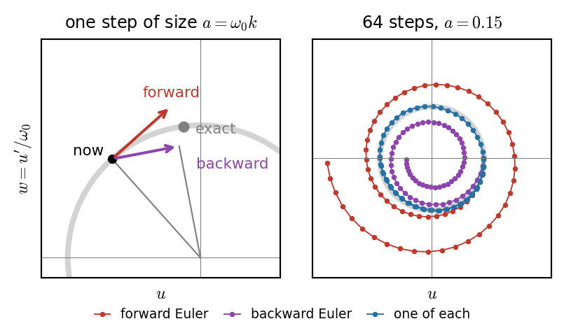
- Forward: move along the tangent at the start.
Radius \(\times\sqrt{1+a^2}\). - Backward: move along the tangent at the arrival.
Radius \(\div\sqrt{1+a^2}\).
Remark. Numerical Damping
- A force one step late or early acts like friction:
\(u^{n\mp1}\approx u\mp k\,u'\ \Rightarrow\ u''\,{\color{firebrick}{\mp\,\omega_0^2k\,u'}}+\omega_0^2u=0\) - It vanishes as \(k\to0\), but only as \(O(k)\).
440 Hz at 44.1 kHz: \(\times\,5700\) or \(\div\,5700\) in 0.1 s.
Keeping Difference Quantities w/o Differentiating
- Sometimes you want to control variables that are defined by derivatives.
- e.g., preserving the invariants (curvature of clothes, divergence of fluid flow, …)
- Approaching it by computing with finite differences: Is only correct in the limit \(h\to0\).
The fundamental theorem of calculus is exact for any spacing
\[ \int_{t_i}^{t_{i+1}} f'(t)\,dt = f(t_{i+1})-f(t_i) \]
and the choice of \(h\) does not matter here. A difference of samples is the exact value of an integrated derivative.
Example: Structure-Preserving Discretization
- Curvature \(\kappa\) of a scanned outline is a second derivative quantity.
- For a smooth closed curve, \(\oint\kappa\,ds=2\pi\) (cf. Gauss-Bonnet theorem).
- On a polygon, define the integrated curvature at a vertex as its turning angle \(\theta_i\). Then
\[\sum_i\theta_i=2\pi\quad\text{exactly, for any number of points.}\]
You can manipulate the polygonal curve while preserving the total curvature, without ever computing a derivative.
On the other hand, if you compute curvature from finite differences of the coordinates, you get a number that converges to \(2\pi\) only as \(h\to0\).
Example. The finite difference approximation of curvature is not exact for large \(h\).
Show code
def outline(n):                                         # n samples of a smooth closed curve
    s = 2 * np.pi * np.arange(n) / n
    r = 1 + 0.25 * np.cos(3 * s) + 0.15 * np.sin(2 * s)
    return np.stack([r * np.cos(s), r * np.sin(s)], 1)

def total_turning(P):                                   # sum of the turning angles of the polygon
    e = np.roll(P, -1, 0) - P
    e_prev = np.roll(e, 1, 0)
    cross = e_prev[:, 0] * e[:, 1] - e_prev[:, 1] * e[:, 0]
    return np.sum(np.arctan2(cross, np.sum(e_prev * e, 1)))

def total_fd_curvature(P):                              # curvature from centered differences, then summed
    d1 = (np.roll(P, -1, 0) - np.roll(P, 1, 0)) / 2
    d2 = np.roll(P, -1, 0) - 2 * P + np.roll(P, 1, 0)
    speed = np.hypot(d1[:, 0], d1[:, 1])
    kappa = (d1[:, 0] * d2[:, 1] - d1[:, 1] * d2[:, 0]) / speed**3
    return np.sum(kappa * speed)

fig, axs = plt.subplots(1, 2, figsize=(4.5, 4.4), width_ratios=[1, 1.15])
fine, P = outline(400), outline(10)
axs[0].plot(*np.vstack([fine, fine[:1]]).T, color="lightgray", lw=3)
axs[0].plot(*np.vstack([P, P[:1]]).T, "-o", color="steelblue", ms=4, lw=1.5)
axs[0].set_aspect("equal"); axs[0].axis("off")
axs[0].set_title("scanned outline, 10 points", fontsize=9)

ns = np.array([6, 8, 12, 16, 24, 32, 48, 64, 96, 128])
axs[1].loglog(ns, [abs(total_fd_curvature(outline(n)) - 2 * np.pi) for n in ns], "-o", ms=3, color="firebrick", label="differenced curvature")
axs[1].loglog(ns, [max(abs(total_turning(outline(n)) - 2 * np.pi), 1e-16) for n in ns], "-o", ms=3, color="steelblue", label="turning angles")
axs[1].set_xlabel("number of points"); axs[1].set_title("$|\\,$total curvature $-\\,2\\pi\\,|$", fontsize=9)
axs[1].set_ylim(1e-17, 10)
axs[1].legend(fontsize=7, loc="center right")
plt.tight_layout()
plt.show()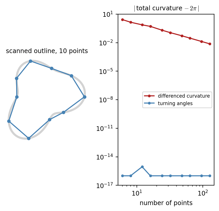
Structure Preservation: Does the Outline Close?
Test: throw away the coordinates of the 10 point outline. Keep only the edge lengths and the curvature at each vertex, then walk the outline again: go straight along an edge, turn by the stored curvature, repeat.
Show code
def turning_angles(P):                                  # angle between consecutive edges, at every vertex
    e = np.roll(P, -1, 0) - P
    e_prev = np.roll(e, 1, 0)
    cross = e_prev[:, 0] * e[:, 1] - e_prev[:, 1] * e[:, 0]
    return np.arctan2(cross, np.sum(e_prev * e, 1))

def differenced_angles(P):                              # differenced curvature times the local arc length
    d1 = (np.roll(P, -1, 0) - np.roll(P, 1, 0)) / 2
    d2 = np.roll(P, -1, 0) - 2 * P + np.roll(P, 1, 0)
    return (d1[:, 0] * d2[:, 1] - d1[:, 1] * d2[:, 0]) / (d1[:, 0]**2 + d1[:, 1]**2)

def rebuild(P, angles):                                 # walk the same edge lengths, turning by angles[i] at vertex i
    e = np.roll(P, -1, 0) - P
    length = np.hypot(e[:, 0], e[:, 1])
    heading = np.arctan2(e[0, 1], e[0, 0]) + np.concatenate([[0], np.cumsum(angles[1:])])
    steps = length[:, None] * np.stack([np.cos(heading), np.sin(heading)], 1)
    return P[0] + np.concatenate([np.zeros((1, 2)), np.cumsum(steps, 0)])

P = outline(10)
closed = np.vstack([P, P[:1]])
th_turn, th_fd = turning_angles(P), differenced_angles(P)

fig, axs = plt.subplots(1, 3, figsize=(9, 2.8), width_ratios=[1.25, 1, 1])
i = np.arange(len(P))
axs[0].bar(i - 0.2, th_fd, 0.4, color="firebrick",
           label=f"differenced $\\kappa_i\\,\\Delta s_i$: sum $=2\\pi+{th_fd.sum() - 2 * np.pi:.2f}$")
axs[0].bar(i + 0.2, th_turn, 0.4, color="steelblue", label="turning angle $\\theta_i$: sum $=2\\pi$")
axs[0].axhline(0, color="k", lw=0.5)
axs[0].set_xticks(i); axs[0].set_xlabel("vertex $i$"); axs[0].set_ylabel("integrated curvature (rad)")
axs[0].set_ylim(-0.6, 2.9)
axs[0].set_title("curvature stored at each vertex", fontsize=9)
axs[0].legend(fontsize=7, loc="upper center")

for ax, th, col, ttl in [(axs[1], th_fd, "firebrick", "rebuilt from differenced curvature"),
                         (axs[2], th_turn, "steelblue", "rebuilt from turning angles")]:
    Q = rebuild(P, th)
    gap = np.hypot(*(Q[-1] - Q[0]))                     # distance between the last point and the first
    ax.plot(*closed.T, color="lightgray", lw=4)
    ax.plot(*Q.T, "-o", color=col, ms=4, lw=1.5)
    ax.plot(*Q[0], "o", color="k", ms=6)
    ax.text(*(Q[0] + [0.08, 0.0]), "start", fontsize=8, va="center")
    if gap > 1e-9:
        ax.plot(*np.stack([Q[-1], Q[0]]).T, color="k", ls=":", lw=1)
        ax.plot(*Q[-1], "s", color=col, ms=6)
        ax.text(*(Q[-1] + [0.0, 0.1]), "end", color=col, fontsize=8, ha="center")
        ax.text(0.5, 0.02, f"does not close: gap {gap:.2f}", transform=ax.transAxes, ha="center", fontsize=8)
    else:
        ax.text(0.5, 0.02, f"closes: gap {gap:.0e}", transform=ax.transAxes, ha="center", fontsize=8)
    ax.set_xlim(-1.5, 1.75); ax.set_ylim(-1.75, 1.45)
    ax.set_aspect("equal"); ax.axis("off")
    ax.set_title(ttl, fontsize=9)
plt.tight_layout()
plt.show()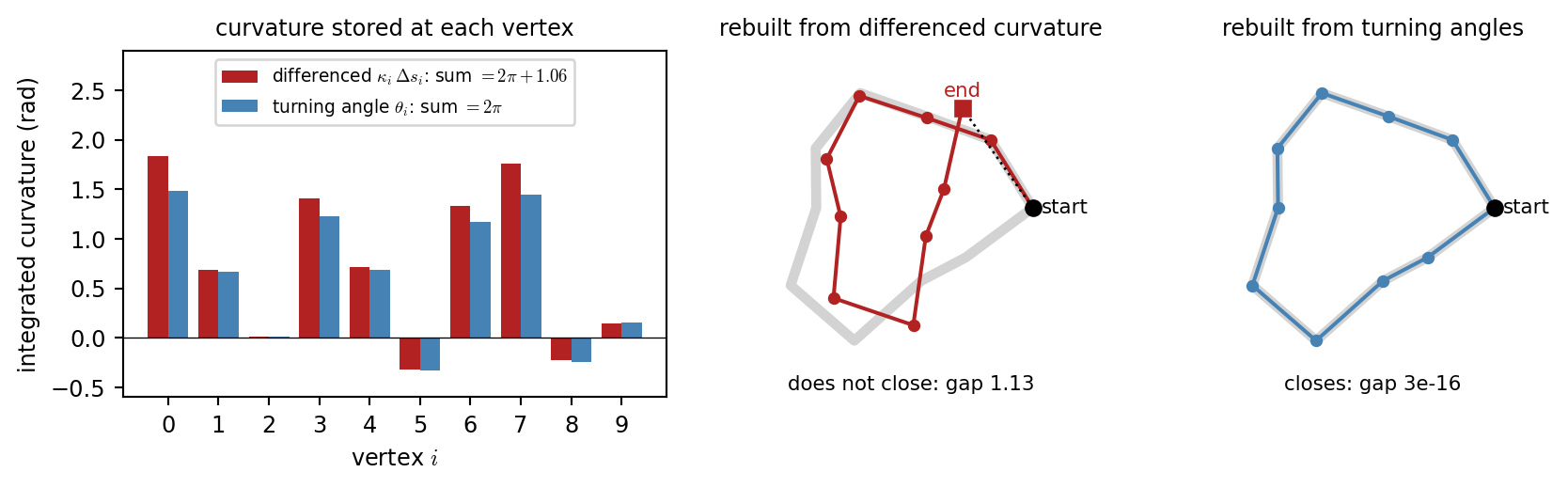
Violation. Differenced curvature is too large at every sharp vertex.
- The errors add up: the tangent turns \(2\pi+1.06\), about \(61^\circ\) too far.
- The rebuilt outline does not close: \(\oint\kappa\,ds=2\pi\) is broken.
- More points shrink the gap, but never remove it.
Fix: preserve the angles. Store the turning angle \(\theta_i\) between consecutive edges.
- \(\sum_i\theta_i=2\pi\) exactly: the tangent returns to its start.
- The rebuilt outline is the original polygon, even with 10 points.
- Same idea as the oscillator scheme that conserves \(\mathfrak{h}^n\) exactly.