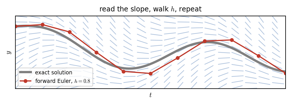
Ordinary Differential Equations I
Topics in Digital Heritage:
Numerical Methods for Digital Reconstruction
Fall 2026
What Exactly Is an ODE?
An ODE (Ordinary Differential Equation) relates an unknown function to its derivatives, e.g. \(u''(t)=-\omega_0^2u(t)\).
- Ordinary: one independent variable, time \(t\).
- Partial (PDE, next week): \(u(x,t)\) with \(\partial_x\) and \(\partial_t\). After discretizing space, a PDE becomes a large ODE system.
| term | meaning | example |
|---|---|---|
| order | highest derivative | SHO: 2nd order |
| system | vector unknown \(\mathbf{y}\) | \((u,u')\); \(N\) masses |
| linear | \(F\) linear in \(\mathbf{y}\) | \(\mathbf{y}'=A\mathbf{y}\) |
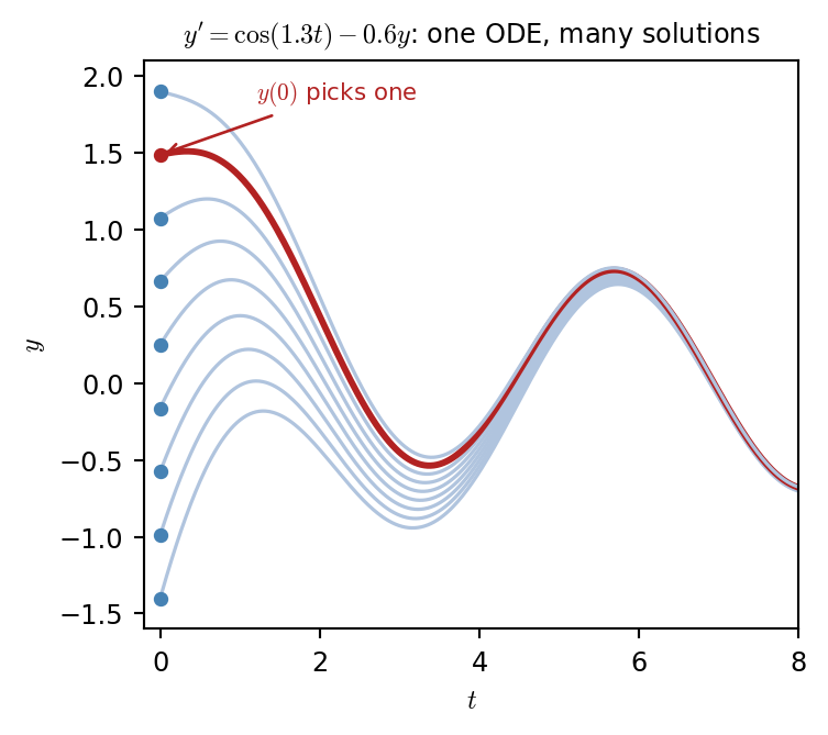
Remark. An ODE fixes slopes, not a single curve
- Solutions form a family. An initial value \(\mathbf{y}(0)\) picks one: the initial value problem.
- Closed forms are rare (\(y'=\lambda y\Rightarrow y=y_0e^{\lambda t}\)). Nonlinear or large systems need time stepping.
ODEs Are Everywhere
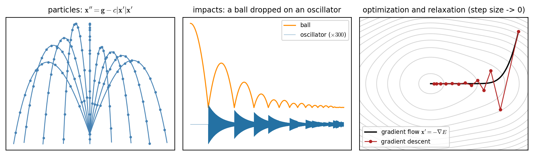
And many more: cloth, hair, rigid bodies, crowds, molecules, the circuits of analog synthesizers.
Each one is a state that changes by a rule.
The common thread: an initial value problem
- Given the state \(\mathbf{y}(0)\)
- and a rule \(\mathbf{y}'=F(t,\mathbf{y})\) for its rate of change,
- predict \(\mathbf{y}(t)\) for \(t>0\).
Setting Up an Initial Value Problem
Find \(\mathbf{y}(t)\in\mathbb{R}^n\) such that
\[ \mathbf{y}'(t)=F\bigl(t,\mathbf{y}(t)\bigr),\qquad \mathbf{y}(0)=\mathbf{y}_0 . \]
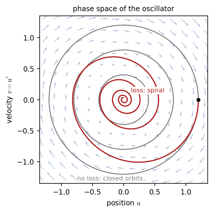
Any explicit ODE becomes first order by adding variables. For the damped oscillator:
\[\begin{align} u''&=-\omega_0^2u-2\sigma_0u' \\ \Longrightarrow \frac{d}{dt}\begin{pmatrix}u\\ u'\end{pmatrix} &=\begin{pmatrix} 0&1\\-\omega_0^2&-2\sigma_0\end{pmatrix}\begin{pmatrix}u\\ u'\end{pmatrix} \\ \boxed{\mathbf{y}'=A \mathbf{y}}\qquad A &= \begin{pmatrix}0&1\\-\omega_0^2&-2\sigma_0\end{pmatrix},\ \mathbf{y}=\begin{pmatrix}u\\ u'\end{pmatrix} \end{align}\]
From the box to an integral
Integrate both sides over one step \([t,t+h]\). The fundamental theorem of calculus turns the left side into a difference.
\[ \begin{aligned} \int_t^{t+h}\mathbf{y}'(s)\,ds&=\int_t^{t+h}A\,\mathbf{y}(s)\,ds\\ \mathbf{y}(t+h)-\mathbf{y}(t)&=\int_t^{t+h}A\,\mathbf{y}(s)\,ds \end{aligned} \]
Exact, but needs the unknown \(\mathbf{y}(s)\). In general, \(A\mathbf{y}\to F(s,\mathbf{y}(s))\).
One Step Is One Integral
\[ \mathbf{y}_{k+1}=\mathbf{y}_k+\int_{t_k}^{t_k+h}F\bigl(s,\mathbf{y}(s)\bigr)\,ds \]
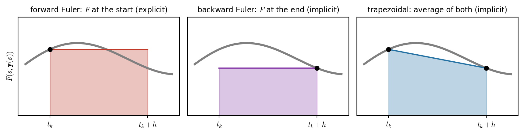
Apply a quadrature rule to the integral:
| Rule | Method | Update |
|---|---|---|
| left endpoint | forward Euler | \(\mathbf{y}_{k+1}=\mathbf{y}_k+hF(\mathbf{y}_k)\) |
| right endpoint | backward Euler | \(\mathbf{y}_{k+1}=\mathbf{y}_k+hF(\mathbf{y}_{k+1})\) |
| trapezoid | trapezoidal | \(\mathbf{y}_{k+1}=\mathbf{y}_k+\tfrac{h}{2}\bigl[F(\mathbf{y}_k)+F(\mathbf{y}_{k+1})\bigr]\) |
Accuracy: one step versus the whole run
Local error (one step) \(\times\) number of steps \(T/h\) \(=\) global error: Euler \(O(h^2)\to O(h)\), trapezoidal \(O(h^3)\to O(h^2)\). Same as composite quadrature (class 9), and the same as \(\delta_{t+}\mathbf{y}=F\) and \(\delta_{t-}\mathbf{y}=F\) (class 10).
Checking the Order of Accuracy Ourselves
Show code
T = 2.0
hs = 2.0 ** -np.arange(3, 12)
y_T = exact_osc(T)
methods = {
    "forward Euler": lambda y, h: y + h * A_osc @ y,
    "backward Euler": lambda y, h: backward_euler_lin(A_osc, y, h),
    "trapezoid": lambda y, h: trapezoid_lin(A_osc, y, h),
}

fig, axs = plt.subplots(1, 2, figsize=(9, 3.3))
for name, step in methods.items():
    err = []
    for h in hs:
        y = y0_osc.copy()
        for _ in range(int(round(T / h))):
            y = step(y, h)
        err.append(np.linalg.norm(y - y_T))
    err = np.array(err)
    p = np.polyfit(np.log(hs[-5:]), np.log(err[-5:]), 1)[0]          # slope for small h
    axs[0].loglog(hs, err, "-o", ms=3, color=COL[name], label=f"{name}: slope {p:.2f}")
axs[0].set_xlabel("time step $h$"); axs[0].set_ylabel("$\\|\\mathbf{y}_n-\\mathbf{y}(2)\\|$")
axs[0].set_title("damped oscillator, error at $t=2$", fontsize=9)
axs[0].legend(fontsize=8)

h = 0.1
tt = np.linspace(0, 6, 600)
axs[1].plot(tt, [exact_osc(t)[0] for t in tt], color="gray", lw=3, label="exact")
for name, step in methods.items():
    Y = [y0_osc]
    for _ in range(60):
        Y.append(step(Y[-1], h))
    u = np.array(Y)[:, 0]
    if np.any(np.abs(u) > 2.2):                                       # stop drawing once it leaves the plot
        u[np.argmax(np.abs(u) > 2.2) + 1:] = np.nan
    axs[1].plot(h * np.arange(61), u, "-o", ms=2, lw=1, color=COL[name], label=name)
axs[1].set_xlabel("$t$"); axs[1].set_ylabel("$u$"); axs[1].set_ylim(-2.2, 2.2)
axs[1].set_title(f"same order, different character ($h={h}$)", fontsize=9)
axs[1].legend(fontsize=7, ncol=2, loc="lower left")
plt.tight_layout()
plt.show()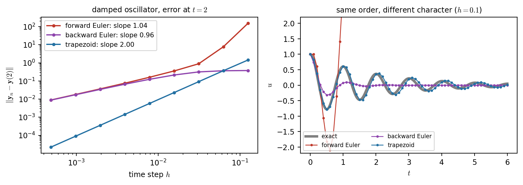
Order is not the whole story
Order tells us how fast the error shrinks. It does not tell us whether the solution blows up.
When Does a Method Blow Up?
Consider the model equation \(y'=\lambda y\).
Apply a method: e.g., forward Euler \(\Rightarrow y_{k+1}=y_k+h\lambda y_k\).
- Every step multiplies by the same number, e.g. \(z := h\lambda\).
- Denote this number by \(R(z)\) (called “amplification factor”). \[ y_{k+1}=R(z)\,y_k\ \Rightarrow\ y_k=R(z)^k\,y_0,\qquad \text{exact: }R=e^{z} \]
| \(R(z)\) | stable (\(\lvert R\rvert\le1\)) | |
|---|---|---|
| forward Euler | \(1+z\) | disk around \(-1\) |
| backward Euler | \(1/(1-z)\) | outside disk around \(+1\) |
| trapezoid | \((1+z/2)/(1-z/2)\) | left half plane |
Remark. Reading the regions
- Decay (\(\lambda<0\)): forward Euler needs \(h<2/\lvert\lambda\rvert\).
- Gradient descent is forward Euler on \(\mathbf{x}'=-\nabla E\): the learning rate limit \(h<2/L\) (class 7) is this condition.
- Oscillators (\(\lambda=\pm j\omega\)) on the imaginary axis:
- forward Euler: always grows,
- backward Euler: always decays,
- trapezoid: \(\lvert R\rvert=1\) exactly, but \(\arg R\neq\omega h\) (pitch error).
- Trapezoid rule = bilinear transform in DSP.
Show code
x, y = np.meshgrid(np.linspace(-3.2, 3.2, 500), np.linspace(-2.6, 2.6, 400))
Z = x + 1j * y
fig, axs = plt.subplots(1, 3, figsize=(9, 2.2))
for ax, name in zip(axs, ["forward Euler", "backward Euler", "trapezoid"]):
    stable = np.abs(R[name](Z)) <= 1
    ax.contourf(x, y, stable, levels=[0.5, 1.5], colors=[COL[name]], alpha=0.25)
    ax.contour(x, y, np.abs(R[name](Z)), levels=[1], colors=[COL[name]], linewidths=1.5)
    ax.axhline(0, color="gray", lw=0.5); ax.axvline(0, color="k", lw=1.5)
    ax.set_aspect("equal"); ax.set_xticks([-2, 0, 2]); ax.set_yticks([-2, 0, 2])
    ax.set_xlabel("Re $z$"); ax.set_title(f"{name}: shaded = stable", fontsize=9)
axs[0].set_ylabel("Im $z$")
plt.tight_layout()
plt.show()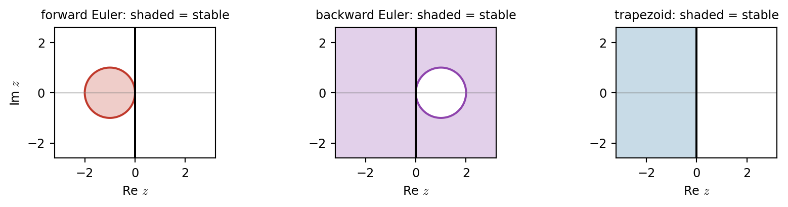
Systems with Multiple Eigenvalues
Stiff Spring Network: The Fastest Mode Sets the Step
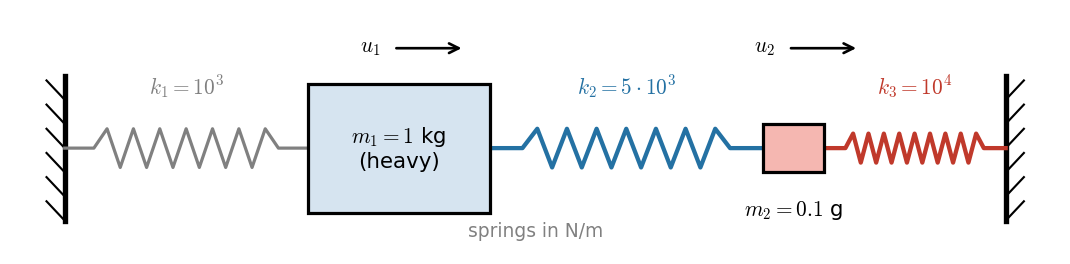
\[ M\mathbf{u}''=-K\mathbf{u},\quad M=\begin{pmatrix}m_1& 0 \\ 0 & m_2\end{pmatrix},\quad K=\begin{pmatrix}k_1+k_2&-k_2\\-k_2&k_2+k_3\end{pmatrix} \]
Modes: 10.5 Hz (the motion we want) and 1950 Hz (a tiny, fast jiggle). Explicit methods need \(h\lambda\) inside the region for every eigenvalue.
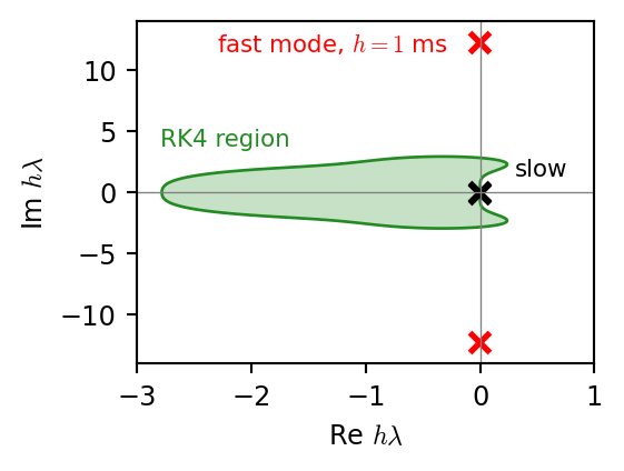
An explicit method must take tiny steps for stability, not for accuracy. Implicit methods take any \(h\): backward Euler erases the fast mode, the trapezoid keeps it as a zigzag (\(R\to-1\)).
Stiffness in Practice: Explicit or Implicit at 1 ms
Show code
y0_st = np.array([0.01, 0.0, 0.0, 0.0])                 # pull the heavy mass, release
F_st = lambda t, y: A_st @ y
T_st = 0.25
t_ref = np.linspace(0, T_st, 2000)
Y_ref = np.array([expm(A_st * t) @ y0_st for t in t_ref])
runs = [("RK4, $h=1$ ms", lambda y, h: rk4(F_st, 0, y, h), 1e-3, COL["RK4"], "-"),
("RK4, $h=0.2$ ms", lambda y, h: rk4(F_st, 0, y, h), 2e-4, "darkgreen", ":"),
        ("backward Euler, $h=1$ ms", lambda y, h: backward_euler_lin(A_st, y, h), 1e-3, COL["backward Euler"], "-"),
        ("trapezoid, $h=1$ ms", lambda y, h: trapezoid_lin(A_st, y, h), 1e-3, COL["trapezoid"], "-")]
fig, axs = plt.subplots(1, 2, figsize=(9, 2.1))
axs[0].plot(t_ref, Y_ref[:, 0], color="gray", lw=3)
axs[1].plot(t_ref, Y_ref[:, 1], color="lightgray", lw=1, label="exact")
for lab, step, h, col, ls in runs:
    Y = [y0_st]
    for _ in range(int(round(T_st / h))):
        Y.append(step(Y[-1], h))
    Y = np.array(Y); tk = h * np.arange(len(Y))
    if np.any(np.abs(Y[:, 0]) > 0.015):                      # stop drawing once it leaves the plot
        Y[np.argmax(np.abs(Y[:, 0]) > 0.015) + 1:] = np.nan
    axs[0].plot(tk, Y[:, 0], color=col, ls=ls, lw=1.3, label=lab)
    if "RK4, $h=1" not in lab:
        lw = 1.8 if "RK4" in lab else 1.2
        axs[1].plot(tk, Y[:, 1], "-o" if h == 1e-3 else ls, color=col, ms=3, lw=lw, label=lab)
axs[0].set_ylim(-0.015, 0.015); axs[0].set_title("heavy mass $u_1$ (RK4 at 1 ms leaves the plot)", fontsize=9)
axs[1].set_xlim(0, 0.03); axs[1].set_ylim(-0.012, 0.012); axs[1].set_title("light mass $u_2$, first 30 ms", fontsize=9)
axs[0].legend(fontsize=6.5, loc="lower left", ncol=2)
for ax in axs:
    ax.set_xlabel("$t$ (s)")
plt.tight_layout()
plt.show()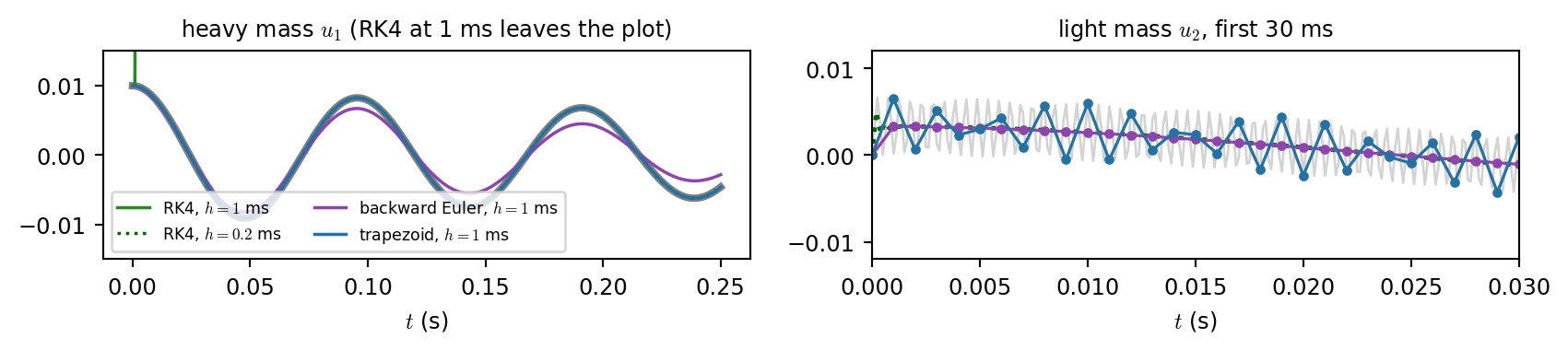
Runge-Kutta: Higher Order Without Solving
Heun: trapezoid rule, with \(\mathbf{y}_{k+1}\) predicted by a forward Euler step (error \(O(h^2)\cdot h\), harmless).
\[ \mathbf{y}_{k+1}=\mathbf{y}_k+\tfrac{h}{2}\Bigl[F(\mathbf{y}_k)+F\bigl(\underbrace{\mathbf{y}_k+hF(\mathbf{y}_k)}_{\text{predict}}\bigr)\Bigr] \]
RK4: the same idea built on Simpson’s rule.
Weights \(\tfrac16(1,2,2,1)\): Simpson’s \(\tfrac16(1,4,1)\) with the midpoint used twice.
| \(F\) per step | order | |
|---|---|---|
| forward Euler | 1 | 1 |
| Heun | 2 | 2 |
| RK4 | 4 | 4 |
Show code
x, y = np.meshgrid(np.linspace(-3.4, 1.2, 500), np.linspace(-3.4, 3.4, 500))
Z = x + 1j * y
fig, ax = plt.subplots(figsize=(4.3, 3.7))
for name in ["RK4", "Heun", "forward Euler"]:
    ax.contourf(x, y, np.abs(R[name](Z)) <= 1, levels=[0.5, 1.5], colors=[COL[name]], alpha=0.18)
    ax.contour(x, y, np.abs(R[name](Z)), levels=[1], colors=[COL[name]], linewidths=1.5)
    ax.plot([], [], color=COL[name], label=name)
ax.axhline(0, color="gray", lw=0.5); ax.axvline(0, color="k", lw=1.5)
ax.plot([0, 0], [-2.83, 2.83], color=COL["RK4"], lw=4, alpha=0.6)
ax.text(0.1, 2.9, "$\\pm2.83j$", color=COL["RK4"], fontsize=8)
ax.set_aspect("equal"); ax.set_xlabel("Re $z$"); ax.set_ylabel("Im $z$")
ax.set_title("$R(z)$ = Taylor series of $e^z$, truncated", fontsize=9)
ax.legend(fontsize=7, loc="lower left")
plt.tight_layout()
plt.show()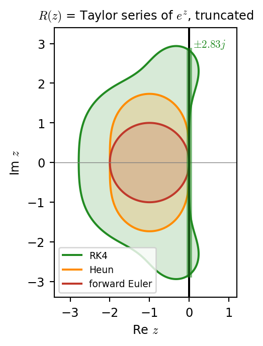
Remark. Bigger, but still bounded
RK4 covers part of the imaginary axis: explicit and stable for oscillators if \(\omega h<2.83\). But \(R(z)\) is a polynomial, so every explicit region is bounded.
Inside One Runge-Kutta Step
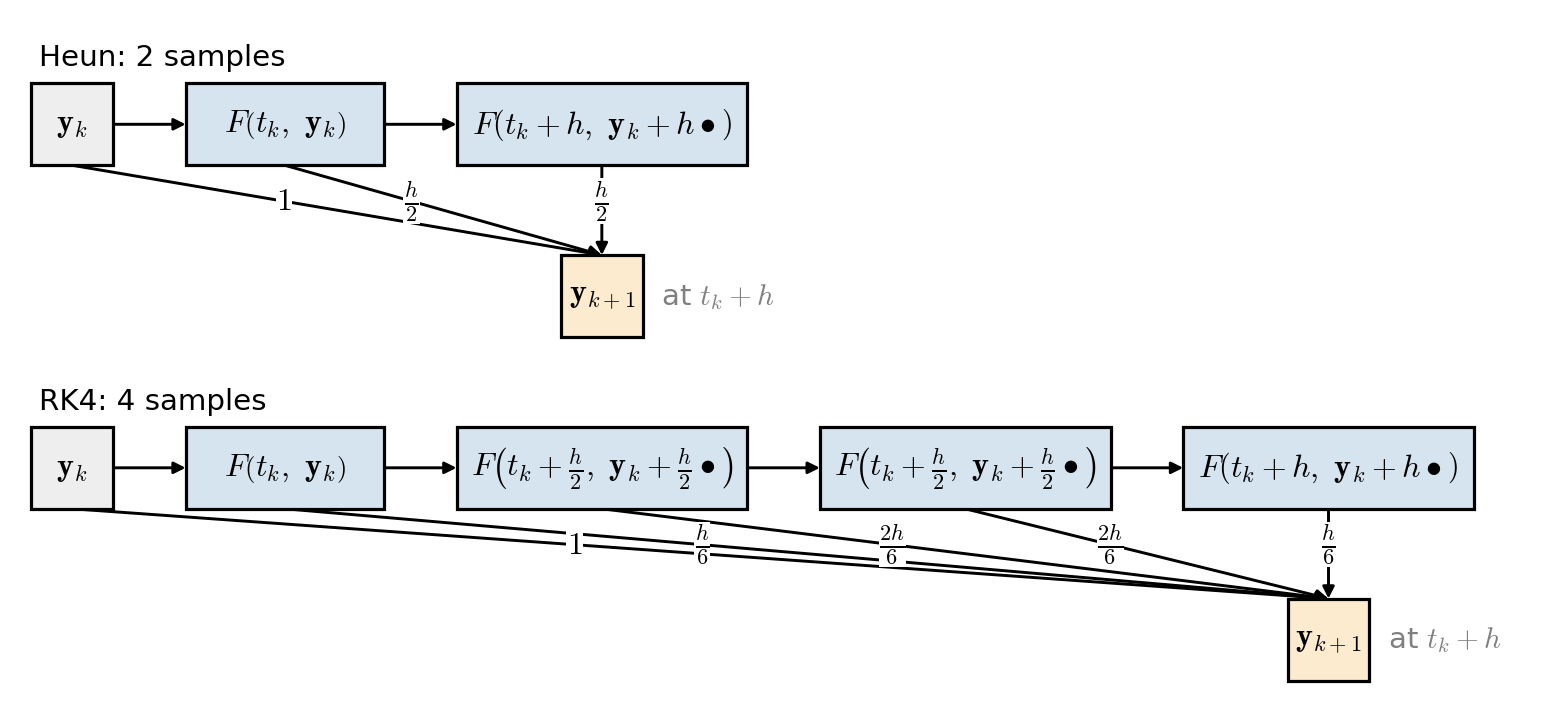
Row (samples): in evaluation order; \(\bullet\) is the value on the incoming arrow (the previous \(F\)), and every sample starts from \(\mathbf{y}_k\).
Down (output): a weighted sum of the \(F\) values at the end of the step; the weights are the quadrature weights.
Causality = explicit
Every arrow points right or down: a sample only uses samples already computed. An arrow pointing back (backward Euler: \(F(\mathbf{y}_{k+1})\) feeds \(\mathbf{y}_{k+1}\)) means an equation to solve, i.e. an implicit method.
Getting the Most Accuracy per Evaluation
Show code
T = 5.0
y_T = exact_osc(T)
fig, ax = plt.subplots(figsize=(4.4, 3.4))
for name, step, cost in [("forward Euler", euler, 1), ("Heun", heun, 2), ("RK4", rk4, 4)]:
    ns = np.unique(np.geomspace(60, 40000, 12).astype(int))
    err = [np.linalg.norm(integrate(step, F_osc, y0_osc, T / n, n)[-1] - y_T) for n in ns]
    ax.loglog(cost * ns, err, "-o", ms=3, color=COL[name], label=f"{name} ({cost} per step)")
ax.axhline(1e-6, color="gray", ls=":", lw=1)
ax.set_xlabel("number of $F$ evaluations"); ax.set_ylabel("error at $t=5$")
ax.set_ylim(1e-12, 1e2)
ax.set_title("damped oscillator: work vs accuracy", fontsize=9)
ax.legend(fontsize=7)
plt.tight_layout()
plt.show()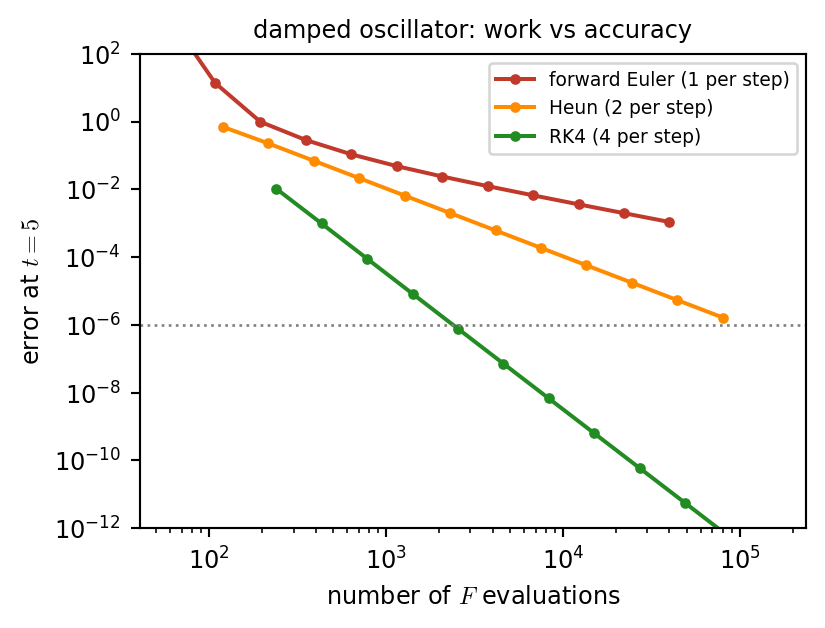
In practice: adaptive step size
Compute each step with two methods of different order, use their difference as an error estimate, then accept or shrink \(h\).
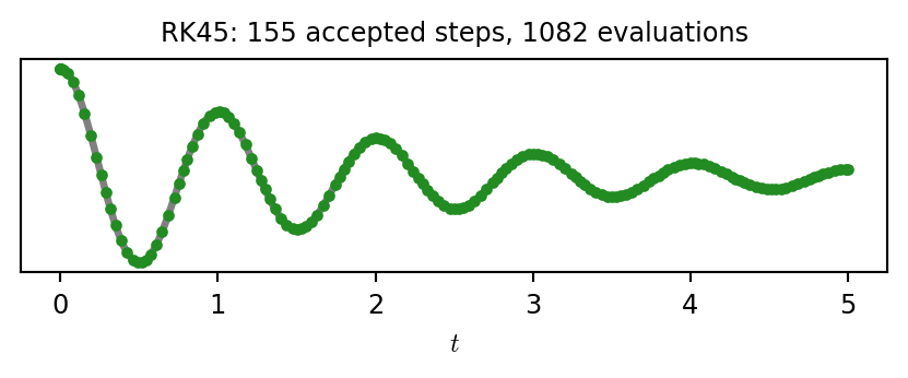
Adaptive Step Size: What Changes
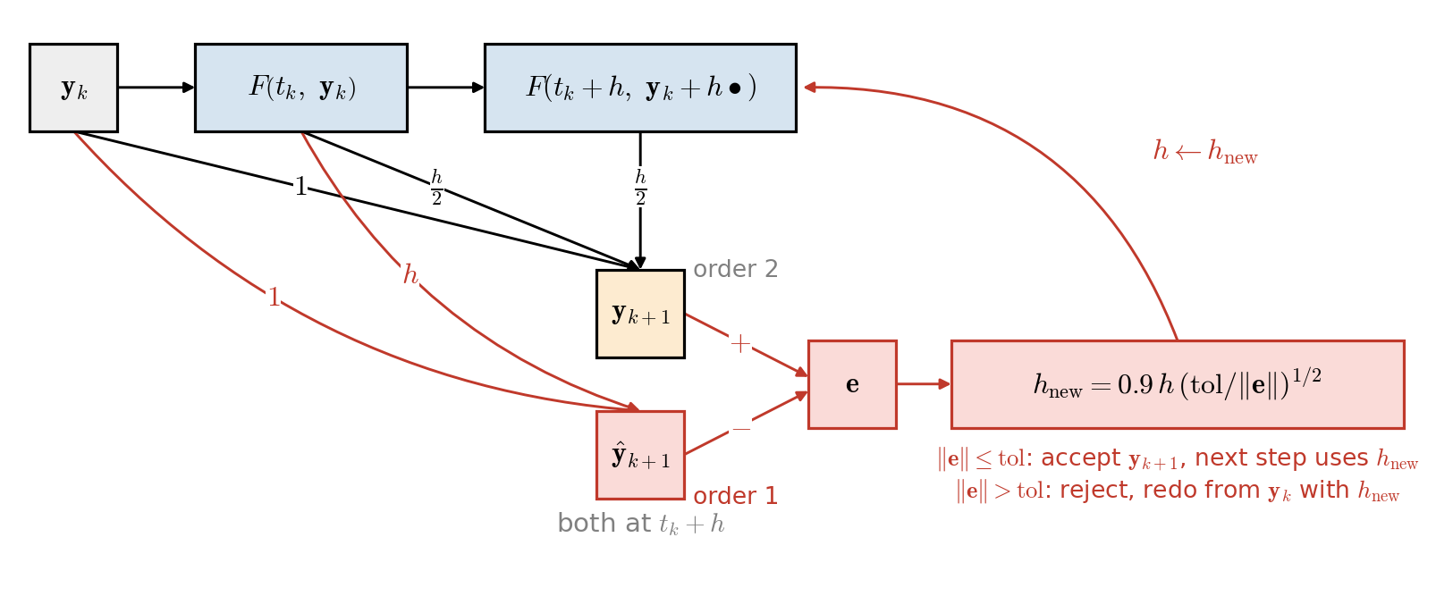
| What changed | Heun–Euler (above) | RK45 in solve_ivp |
|---|---|---|
| second output, same samples | \(\hat{\mathbf{y}}_{k+1}=\mathbf{y}_k+hF(t_k,\mathbf{y}_k)\), the argument of Heun’s 2nd sample | 7 samples, two weight sets |
| error estimate, no extra \(F\) | \(\mathbf{e}=\tfrac{h}{2}\bigl[F(t_k+h,\hat{\mathbf{y}}_{k+1})-F(t_k,\mathbf{y}_k)\bigr]\) | order 5 \(-\) order 4 |
| step-size exponent \(1/(p+1)\) | \(1/2\) | \(1/5\), with \(\mathrm{tol}=\texttt{atol}+\texttt{rtol}\,\lvert\mathbf{y}\rvert\) |
Damped Harmonic Oscillator
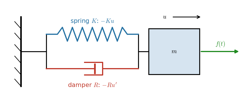
Newton’s second law
\[ m\,u''=\underbrace{-K\,u}_{\text{spring}}\ \underbrace{-\,R\,u'}_{\text{damper}}\ +\ f(t) \]
- Spring (Hooke): pulls back in proportion to the displacement.
- Damper: resists in proportion to the velocity. Air drag, internal friction, sound radiation.
- \(f(t)\): the external force, e.g. a mallet, or a falling ball (soon)
Divide by \(m\) and name the two constants:
\[ u''=-\omega_0^2\,u-2\sigma_0\,u'+\tfrac{1}{m}f(t),\qquad \omega_0^2=\frac{K}{m},\quad 2\sigma_0=\frac{R}{m} \]
Try \(u=e^{st}\):
\[ s^2+2\sigma_0s+\omega_0^2=0\ \Rightarrow\ s_\pm=-\sigma_0\pm j\omega_1,\quad \omega_1=\sqrt{\omega_0^2-\sigma_0^2} \]
- \(\omega_0\) is the pitch without loss (rad/s): stiffer spring or lighter mass, higher note.
- \(\sigma_0\) is the decay rate of the envelope \(e^{-\sigma_0t}\).
- \(s_\pm\) are the eigenvalues of \(A\) in \(\mathbf{y}'=A\mathbf{y}\): the damped pair in the \(\lambda\) plane.
Remark. The same equation elsewhere
An RLC circuit \(Lq''+Rq'+q/C=V\), and every mode of a spring network, string, or plate.
Application: A Ball on a Damped Oscillator
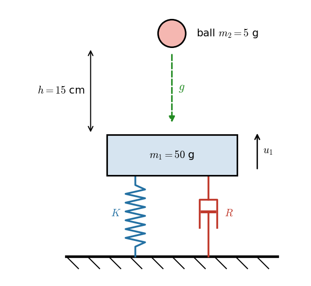
- \(K,R\) tuned so that \(m_1\) rings at \(f_0=400\) Hz with \(T_{60}=1.5\) s: \(\sigma_0/\omega_0\approx0.002\), strongly underdamped.
Up is positive. \(u_1\): \(m_1\) from rest; \(u_2\): height of the ball above \(m_1\)’s resting top.
\(m_1\) is the damped oscillator from before; the ball supplies its force, \(f(t)=-f_c\): \[ m_1u_1''=-Ku_1-Ru_1'-f_c,\qquad m_2u_2''=-m_2g+f_c \]
Contact (Hertz, with a little loss) only while they overlap, \(\delta=u_1-u_2>0\): \[ f_c=k_c\,\delta^{3/2}\,(1+\lambda\,\delta'),\qquad k_c=10^8\ \text{N/m}^{3/2},\ \lambda=0.1\ \text{s/m} \]
State \(\mathbf{y}=(u_1,u_1',u_2,u_2')\): an IVP \(\ \mathbf{y}'=F(\mathbf{y})\), \(\ \mathbf{y}(0)=(0,0,h,0)\).
Remark. Three time scales
Flight between bounces: about \(0.1\) s. One period of \(m_1\): \(2.5\) ms. One contact: about \(0.3\) ms. \(F\) is nonlinear only through \(f_c\).
Solving It: Adaptive Steps Find the Impacts
- The ball hits \(m_1\) at \(t\approx0.17\) s and bounces, lower each time: the impacts speed up, like a ping-pong ball coming to rest.
- Every impact restrikes \(m_1\), which rings in between (note: \(\mu\)m).
What the step controller does
\(h\) is capped in free fall, shrinks to follow the \(400\) Hz ringing, and shrinks again during each contact.
The force \(f(t)\) of the oscillator slide is no longer given: it is an output of the ODE.
Show code
sol_d = solve_ivp(F_drop, (0, 2), y0_d, rtol=1e-8, atol=1e-12, max_step=1e-3, dense_output=True)
t, Y = sol_d.t, sol_d.y.T
fig, axs = plt.subplots(3, 1, figsize=(5.0, 4.0), sharex=True)
axs[0].plot(t, 1e3 * Y[:, 2], color="darkorange", lw=1.2)
axs[0].set_ylabel("ball $u_2$ (mm)")
axs[0].set_title(f"{len(t) - 1} adaptive steps, {len(impacts(t, Y))} impacts", fontsize=9)
axs[1].plot(t, 1e6 * Y[:, 0], color="#2471a3", lw=0.3)
axs[1].set_ylabel("$u_1$ ($\\mu$m)")
axs[2].semilogy(t[1:], np.diff(t), color="k", lw=0.5)
axs[2].set_ylabel("step $h$ (s)"); axs[2].set_ylim(1e-7, 2e-3)
axs[2].set_xlabel("$t$ (s)", labelpad=0); axs[2].set_xlim(0, 2)
plt.tight_layout(pad=0.3)
plt.show()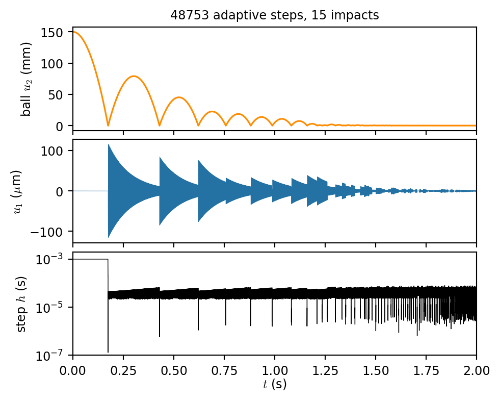
Between Impacts
While the ball is in the air, \(f_c=0\) and \(m_1\) obeys the oscillator equation exactly, so \[ u_1(t)=C\,e^{-\sigma_0t}\cos(\omega_1t+\phi) \] with the same \(\omega_1\) and \(\sigma_0\) as before.
- A contact (\(0.3\) ms) is short against a period (\(2.5\) ms): nearly an impulse \(J=\int f_c\,dt\), which kicks \(u_1'\) by \(-J/m_1\).
- Every bounce restrikes the same oscillator: same pitch \(f_1\approx400\) Hz, same \(T_{60}\). Only \(C\) and \(\phi\) change.
Structure to exploit
A linear oscillator, plus a nonlinear contact that is on for a tiny fraction of the time.
Show code
tz = np.linspace(0, 2, 2_000_001)                                # 1 MHz samples of the dense solution
Yz = sol_d.sol(tz).T
fz = np.array([contact(y) for y in Yz[(tz > 0.16) & (tz < 0.19)]])
tw = tz[(tz > 0.16) & (tz < 0.19)]
J = np.trapezoid(fz, tw); tc = np.trapezoid(tw * fz, tw) / J        # impulse and its centre
w1 = np.sqrt(w0_d**2 - s0_d**2)
fig, axs = plt.subplots(2, 1, figsize=(4.8, 3.6))
m = (tz > tc - 1e-3) & (tz < tc + 15e-3)
ms = 1e3 * (tz[m] - tc)
axs[0].plot(ms, 1e6 * Yz[m, 0], color="k", lw=1.2, label="ODE solution")
te = tz[m] - tc
axs[0].plot(ms[te > 0], -1e6 * J / (m1_d * w1) * np.exp(-s0_d * te[te > 0]) * np.sin(w1 * te[te > 0]),
            color="firebrick", ls="--", lw=1.2, label="oscillator formula, impulse $J$")
env = 1e6 * J / (m1_d * w1) * np.exp(-s0_d * te[te > 0])
axs[0].plot(ms[te > 0], env, color="gray", ls=":", lw=1); axs[0].plot(ms[te > 0], -env, color="gray", ls=":", lw=1)
ax2 = axs[0].twinx(); ax2.fill_between(1e3 * (tw - tc), fz, color="forestgreen", alpha=0.4); ax2.set_ylim(0, 4 * fz.max())
ax2.set_yticks([]); ax2.text(0.6, 0.9 * fz.max(), "$f_c$", color="forestgreen", fontsize=8)
axs[0].set_xlim(-1, 15); axs[0].set_xlabel("time after the first impact (ms)", labelpad=0)
axs[0].set_ylabel("$u_1$ ($\\mu$m)"); axs[0].legend(fontsize=6.5, loc="lower right")
fs = 44100
ts = np.arange(0, 2, 1 / fs); us = sol_d.sol(ts)[0]
U = 20 * np.log10(np.abs(np.fft.rfft(us * np.hanning(len(us)))) + 1e-20); fr = np.fft.rfftfreq(len(us), 1 / fs)
axs[1].semilogx(fr, U - U.max(), color="#2471a3", lw=0.8); axs[1].axvline(f0_d, color="gray", lw=3, alpha=0.4)
axs[1].set_xlim(50, 5000); axs[1].set_ylim(-80, 5)
axs[1].set_xlabel("frequency (Hz)", labelpad=0); axs[1].set_ylabel("dB"); axs[1].set_title("spectrum of $u_1$, all 2 s", fontsize=9)
plt.tight_layout(pad=0.3)
plt.show()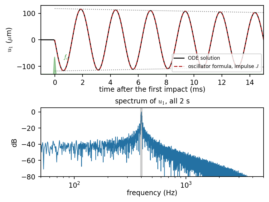
Fixed Steps at an Audio Rate
To make sound we need a value every sample, so \(h=1/f_s\) is fixed. Start times of the impacts for each method (gray: the reference above), and what each one does to the \(400\) Hz oscillator itself:
Show code
def jac_drop(y, K=K_d, R=R_d, kc=kc_d, lam=lam_d):
    d, dd = y[0] - y[2], y[1] - y[3]
    fd = fdd = 0.0
    if d > 0 and 1 + lam * dd > 0:
        fd, fdd = 1.5 * kc * np.sqrt(d) * (1 + lam * dd), lam * kc * d**1.5
    return np.array([[0, 1, 0, 0], [(-K - fd) / m1_d, (-R - fdd) / m1_d, fd / m1_d, fdd / m1_d],
                     [0, 0, 0, 1], [fd / m2_d, fdd / m2_d, -fd / m2_d, -fdd / m2_d]])

def theta_step(y, h, theta, **p):
    """Backward Euler (theta = 1) or trapezoid (theta = 1/2), solved by Newton."""
    Fy = F_drop(0, y, **p); z = y + h * Fy
    for _ in range(30):
        r = z - y - h * (theta * F_drop(0, z, **p) + (1 - theta) * Fy)
        dz = np.linalg.solve(np.eye(4) - h * theta * jac_drop(z, **p), -r)
        z = z + dz
        if np.linalg.norm(dz) < 1e-14 * (1 + np.linalg.norm(z)):
            break
    return z

STEP = {"RK4": lambda y, h, **p: rk4(lambda t, x: F_drop(t, x, **p), 0, y, h),
        "trapezoid": lambda y, h, **p: theta_step(y, h, 0.5, **p),
        "backward Euler": lambda y, h, **p: theta_step(y, h, 1.0, **p),
        "forward Euler": lambda y, h, **p: euler(lambda t, x: F_drop(t, x, **p), 0, y, h)}

def run_fixed(m, fs, T, **p):
    n = int(T * fs); Y = np.full((n + 1, 4), np.nan); Y[0] = y0_d
    with np.errstate(all="ignore"):
        for i in range(n):
            Y[i + 1] = STEP[m](Y[i], 1 / fs, **p)
            if not np.all(np.isfinite(Y[i + 1])) or abs(Y[i + 1, 2]) > 10:
                Y[i + 1:] = np.nan; break
    return np.arange(n + 1) / fs, Y

T = 1.0
runs = [("RK4", 44100), ("RK4", 16000), ("RK4", 8000), ("trapezoid", 44100), ("backward Euler", 44100), ("forward Euler", 44100)]
fig, axs = plt.subplots(1, 2, figsize=(9, 2.9), gridspec_kw=dict(width_ratios=[1.5, 1]))
tr_ = np.linspace(0, T, 1_000_001)
rows = [("reference", impacts(tr_, sol_d.sol(tr_).T), "gray", "")]
for m, fs in runs:
    t_, Y_ = run_fixed(m, fs, T)
    note = "" if np.all(np.isfinite(Y_)) else f"  blows up at {t_[np.argmax(~np.isfinite(Y_[:, 0]))]:.2f} s"
    rows.append((f"{m}, {fs / 1000:g} kHz", impacts(t_, Y_), COL[m], note))
for i, (lab, ti, col, note) in enumerate(rows):
    axs[0].vlines(ti, i - 0.35, i + 0.35, color=col, lw=2)
    if note:
        axs[0].text(T, i, note, ha="right", va="center", fontsize=7, color=col)
axs[0].set_yticks(range(len(rows))); axs[0].set_yticklabels([r[0] for r in rows], fontsize=7); axs[0].invert_yaxis()
axs[0].set_xlim(0, T); axs[0].set_xlabel("$t$ (s)"); axs[0].set_title("rhythm: start time of each impact", fontsize=9)

def numerical_osc(m, fs, w=w0_d, s=s0_d):
    """Pitch error (cents) and T60 ratio a method gives the free oscillator, from its amplification factor."""
    lam = -s + 1j * np.sqrt(w**2 - s**2); z = R[m](lam / fs)
    L = np.log(z) * fs
    return 1200 * np.log2(L.imag / lam.imag), s / -L.real, abs(z)
cells = []
for m, fs in runs:
    c, r, a = numerical_osc(m, fs)
    cells.append([f"{m}, {fs / 1000:g} kHz", "grows" if a > 1 else f"{c:+.2f}", "grows" if a > 1 else f"{r:.2f}"])
axs[1].axis("off")
tb = axs[1].table(cellText=cells, colLabels=["method", "pitch (cents)", "$T_{60}$ ratio"], loc="center", cellLoc="center",
                  colWidths=[0.5, 0.27, 0.23])
tb.auto_set_font_size(False); tb.set_fontsize(7.5); tb.scale(1, 1.35)
axs[1].set_title("the 400 Hz oscillator alone", fontsize=9)
plt.tight_layout()
plt.show()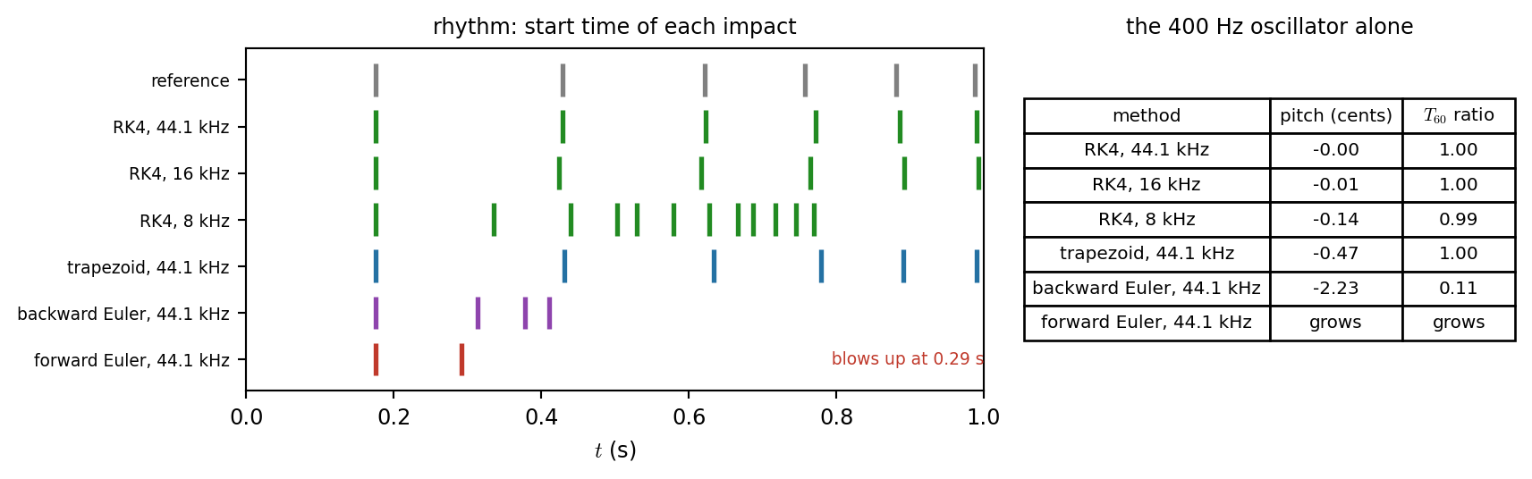
- RK4 keeps the rhythm at \(44.1\) kHz, drifts at \(16\) kHz, loses it at \(8\) kHz: a \(0.3\) ms contact is then only \(2\) to \(3\) samples.
- Forward Euler grows without bound.
- Backward Euler is stable, but takes energy at every impact, and its \(|R| < 1\) cuts the ringing \(T_{60}\) from \(1.5\) s to \(0.17\) s