Partial Differential Equations I
Topics in Digital Heritage:
Numerical Methods for Digital Reconstruction
Fall 2026
PDEs Are Everywhere
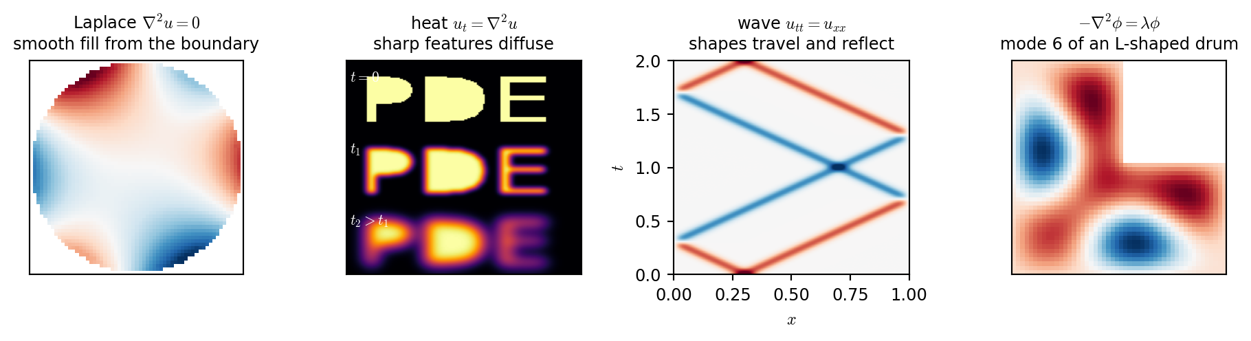
- Graphics: smoke and water (Navier-Stokes), cloth and shells, smooth surface editing (Laplace, biharmonic).
- Audio: strings, bars, drums, plates, tubes, rooms (wave equations).
- Imaging: denoising (heat), CT reconstruction, distance maps (eikonal \(\lVert\nabla d\rVert=1\)).
Anatomy of a PDE Problem
A PDE relates partial derivatives of an unknown function \(u(x,y,\dots,t)\): \[ u_t=\frac{\partial u}{\partial t},\quad u_{xx}=\frac{\partial^2u}{\partial x^2},\quad \nabla^2u=\Delta u=u_{xx}+u_{yy} \]
| PDE | order | linear | where |
|---|---|---|---|
| \(u_t=\alpha u_{xx}\) (heat) | 2 | yes | diffusion, blur |
| \(u_{tt}=\gamma^2u_{xx}\) (wave) | 2 | yes | strings, tubes |
| \(u_{tt}=-\kappa^2u_{xxxx}\) (bar) | 4 | yes | xylophone |
| \(\lVert\nabla d\rVert=1\) (eikonal) | 1 | no | distance maps |
| Navier-Stokes | 2 | no | smoke, water |
- Order: the highest derivative.
- Linear: linear in \(u\) and its derivatives
- the coefficients may still depend on \(x\).
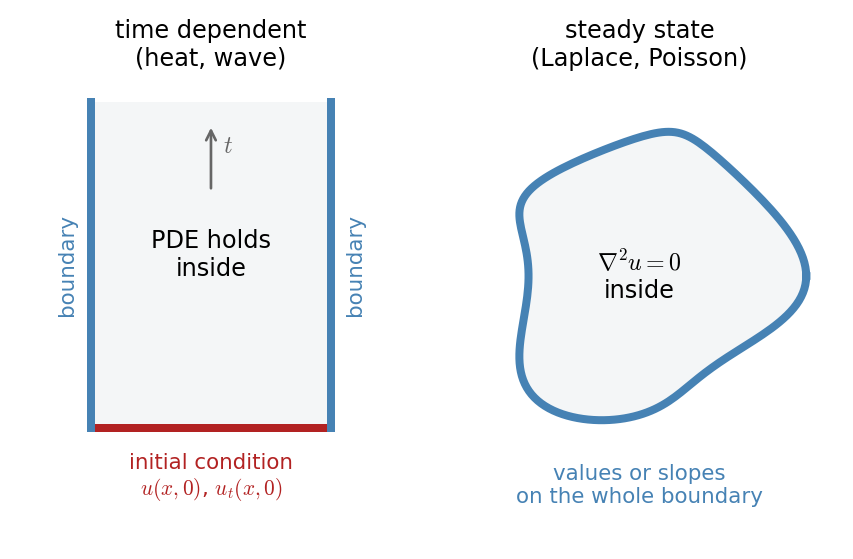
A PDE problem = equation + domain + boundary (+ initial) conditions
ODEs were initial value problems. PDEs are also boundary value problems.
Three Types of Second-Order PDEs
\(a\,u_{xx}+2b\,u_{xy}+c\,u_{yy}+\dots=0\) is classified by the sign of \(D:=b^2-ac\) as:
| type | example | behavior |
|---|---|---|
| elliptic \((D<0)\) | \(\nabla^2u=f\) (Laplace, Poisson) |
equilibrium; every point feels the whole boundary |
| parabolic \((D=0)\) | \(u_t=\alpha\nabla^2u\) (heat) |
smooths and decays; tends to the elliptic solution |
| hyperbolic \((D>0)\) | \(u_{tt}=\gamma^2\nabla^2u\) (wave) |
travels at finite speed, keeps sharp features and energy |
- Heat: curvature sets the velocity, so bumps flatten.
- Wave: curvature sets the acceleration, so bumps overshoot and travel.
- Numerically: a little damping is harmless for heat, but kills a ringing string.
Show code
x = np.linspace(0, 1, 300)
bump = lambda s: np.maximum(0, 1 - np.abs(s - 0.35) / 0.12)          # a narrow pluck
fig, axs = plt.subplots(2, 1, figsize=(4.6, 3.6), sharex=True)
for i, a in enumerate([1, 0.75, 0.5, 0.3]):
    th, tw = [0, 0.0005, 0.002, 0.008][i], [0, 0.1, 0.2, 0.3][i]
    axs[0].plot(x, heat_exact(bump, x, th), color=COL["heat"], alpha=a, lw=1.6, label=f"$t={th:g}$")
    axs[1].plot(x, wave_exact(bump, x, tw), color=COL["wave"], alpha=a, lw=1.6, label=f"$t={tw:g}$")
axs[0].set_title("heat $u_t=u_{xx}$: the corner rounds off, the bump sinks", fontsize=9)
axs[1].set_title("wave $u_{tt}=u_{xx}$: the bump splits and travels, corners stay", fontsize=9)
for ax in axs:
    ax.legend(fontsize=7, ncol=2, loc="upper right"); ax.set_ylim(-0.6, 1.25); ax.set_yticks([0, 1])
axs[1].set_xlabel("$x$")
plt.tight_layout()
plt.show()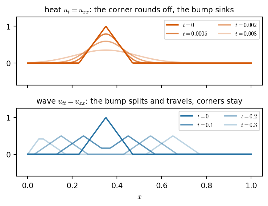
Boundary Conditions
| type | prescribes | examples |
|---|---|---|
| Dirichlet | value \(u\) | nailed string end; intact pixels around a hole |
| Neumann | slope \(\partial u/\partial n\) | end on a sliding ring; insulated end |
| Robin | mix of both | a partly absorbing wall |


Grid Functions and Difference Operators
Grid function: \(u_l^n\approx u(lh,\,nk)\), spacing \(h\), time step \(k\) (\(=1/f_s\) in audio).
| operator | definition | accuracy |
|---|---|---|
| \(\delta_{x+}u_l\) | \(\dfrac{u_{l+1}-u_l}{h}\) | \(O(h)\) |
| \(\delta_{x-}u_l\) | \(\dfrac{u_l-u_{l-1}}{h}\) | \(O(h)\) |
| \(\delta_{x\cdot}u_l\) | \(\dfrac{u_{l+1}-u_{l-1}}{2h}\) | \(O(h^2)\) |
| \(\delta_{xx}=\delta_{x+}\delta_{x-}\) | \(\dfrac{u_{l+1}-2u_l+u_{l-1}}{h^2}\) | \(O(h^2)\) |
| \(\mu_{x+}u_l\) | \(\tfrac12(u_{l+1}+u_l)\) | \(O(h)\) |
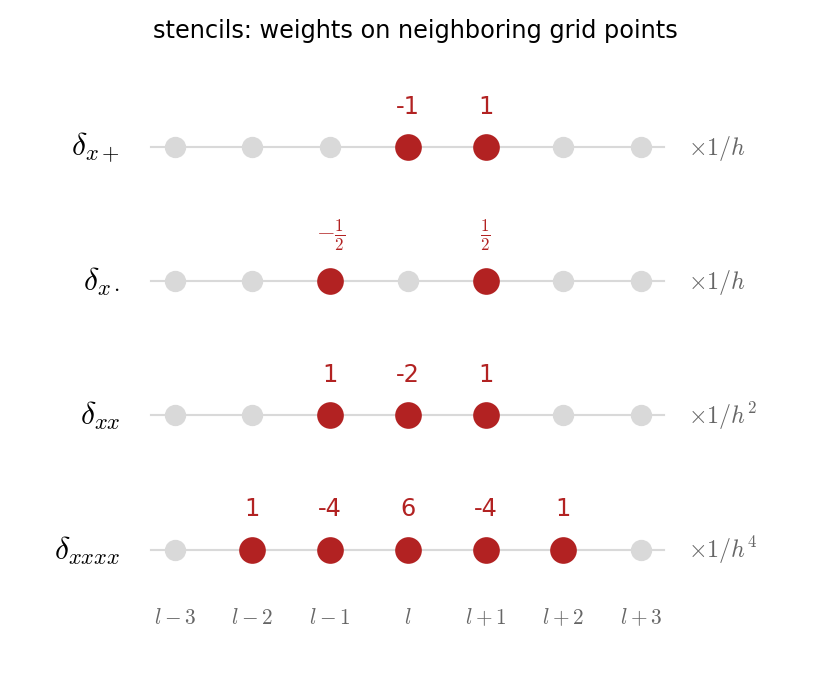
Time operators \(\delta_{t+},\delta_{t-},\delta_{t\cdot},\delta_{tt},\mu_{t\cdot}\) are the same in \(n\) and \(k\).
- Operators compose like algebra: \(\delta_{xxxx}=\delta_{xx}\delta_{xx}\).
- Implement using vectorized operator (e.g., numpy slice):
Operators Are Matrices, Boundaries Are Rows
Dirichlet \(u_0=u_N=0\): drop the known end values; the matrix is just cut.
Neumann \(u_x=0\): the ends are unknowns, and \(\delta_{xx}u_0\) needs \(u_{-1}\), a virtual grid point. Setting \(\delta_{x\cdot}u_0=0\) gives \(u_{-1}=u_1\): \[ \delta_{xx}u_0=\frac{2u_1-2u_0}{h^2} \quad\Rightarrow\quad\text{first row }[-2,\ 2]/h^2 \]
def D_xx_dirichlet(N, h):     # unknowns u_1 .. u_{N-1}
    return sp.diags([1, -2, 1], [-1, 0, 1], shape=(N - 1, N - 1)) / h**2

def D_xx_neumann(N, h):       # unknowns u_0 .. u_N
    D = sp.diags([1, -2, 1], [-1, 0, 1], shape=(N + 1, N + 1)).tolil()
    D[0, 1] = D[N, N - 1] = 2  # virtual points u_{-1} = u_1, u_{N+1} = u_{N-1}
    return D.tocsr() / h**2
The boundary condition is the first and last row. (Symmetric under a trapezoid weighted inner product.)
Show code
def D_xx_neumann(N, h):
    D = sp.diags([1, -2, 1], [-1, 0, 1], shape=(N + 1, N + 1)).tolil()
    D[0, 1] = D[N, N - 1] = 2
    return D.tocsr() / h**2

N = 30; h = 1 / N
eD = np.sort(-np.linalg.eigvals(D_xx(N - 1, h).toarray()).real)
eN = np.sort(-np.linalg.eigvals(D_xx_neumann(N, h).toarray()).real)
fig, ax = plt.subplots(figsize=(4.4, 3.3))
p = np.arange(0, N + 1)
ax.plot(p, p, "k--", lw=1, label="exact: $\\sqrt{-\\lambda_p}/\\pi=p$")
ax.plot(np.arange(1, N), np.sqrt(eD) / np.pi, "o", color="steelblue", ms=4, label="Dirichlet")
ax.plot(p, np.sqrt(np.abs(eN)) / np.pi, "x", color="darkorange", ms=5, label="Neumann (virtual points)")
ax.axhline(2 / (np.pi * h), color="firebrick", lw=0.8, ls=":")
ax.text(1, 2 / (np.pi * h) + 0.5, "spatial Nyquist $2/(\\pi h)$", color="firebrick", fontsize=8)
ax.set_xlabel("mode number $p$"); ax.set_ylabel("$\\sqrt{-\\lambda_p}/\\pi$  (mode frequency)")
ax.set_title(f"eigenvalues of $\\delta_{{xx}}$, $N={N}$: high modes come out low", fontsize=9)
ax.legend(fontsize=7.5, loc="upper left"); ax.set_ylim(0, 33)
plt.tight_layout()
plt.show()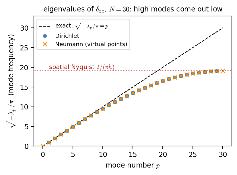
Laplace’s Equation: The Smoothest Fill
Fill a hole \(\Omega\) given the height \(g\) on its boundary, as smoothly as possible: \[ \min_f\int_\Omega\lVert\nabla f\rVert^2\,d\mathbf{x}\ \ \text{s.t.}\ f=g\ \text{on}\ \partial\Omega \ \ \Longrightarrow\ \ \nabla^2f=0 \]
Discrete (5 point Laplacian): each unknown is the average of its 4 neighbors. \[ \tfrac{1}{h^2}\bigl(f_{l+1,m}+f_{l-1,m}+f_{l,m+1}+f_{l,m-1}-4f_{l,m}\bigr)=0 \]
Show code
def lap2d(n, h):                                       # Kronecker sum of two 1D second differences
    D, I = D_xx(n, h), sp.identity(n)
    return (sp.kron(I, D) + sp.kron(D, I)).tocsr()

n = 160; h = 2 / (n - 1)
X, Y, R, z = medallion(n)
hole = ((np.abs(Y - 0.55 * X - 0.1 + 0.05 * np.sin(6 * X)) < 0.05)       # a crack
        | (np.hypot(X - 0.55, Y + 0.55) < 0.22)) & (R < 0.93)             # a chipped edge
U, K = hole.ravel(), ~hole.ravel()                     # unknowns, known (Dirichlet) pixels

def fill(A):                                           # solve A[U,U] f_U = -A[U,K] z_K
    f = z.ravel().copy()
    f[U] = spsolve(A[U][:, U].tocsc(), -A[U][:, K] @ f[K])
    return f.reshape(n, n)

L = lap2d(n, h)
t0 = time.time(); z_lap = fill(L); t_lap = time.time() - t0
z_bih = fill(L @ L)                                    # biharmonic: Laplacian applied twice
fig, axs = plt.subplots(1, 4, figsize=(9.5, 2.75))
damaged = shade(np.where(hole, 0, z), h)
shown = [(damaged, f"damaged ({U.sum()} unknowns)"),
         (shade(z_lap, h), f"Laplace, error {np.abs(z_lap - z)[hole].max():.4f}"),
         (shade(z_bih, h), f"biharmonic, error {np.abs(z_bih - z)[hole].max():.4f}"),
         (shade(z, h), "original")]
for ax, (img, title) in zip(axs, shown):
    ax.imshow(img, cmap="gray", vmin=0); ax.set_title(title, fontsize=8.5); ax.axis("off")
axs[0].contour(hole, levels=[0.5], colors="firebrick", linewidths=0.8)
plt.tight_layout()
plt.show()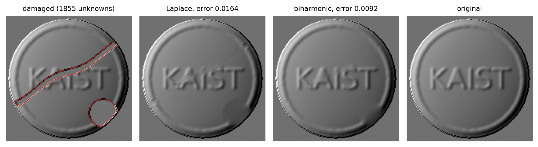
- Laplace matches the values at the edge of the hole; the biharmonic fill also matches the slopes (the plate operator of next class).
- Neither recovers the lost letters: a PDE gives the smoothest guess, not missing information.
Method of Lines: Space First, Then Time
Semidiscretize \(u_t=\alpha u_{xx}\) in space only: \[ \mathbf{u}'(t)=\alpha\,\mathbf{D}_{xx}\,\mathbf{u}(t) \] an ODE system: one ODE per grid point, a line in the \((x,t)\) plane. Then use any integrator of classes 12 and 13.
- Eigenvalues of \(\alpha\mathbf{D}_{xx}\): real, in \(\bigl(-\tfrac{4\alpha}{h^2},0\bigr)\).
- Finer grid \(\Rightarrow\) \(|\lambda_{\max}|\propto1/h^2\): stiff.
- Forward Euler needs \(k|\lambda_{\max}|\le2\): \[ r=\frac{\alpha k}{h^2}\le\frac12 \]
- Halve \(h\): \(4\times\) the steps, \(2\times\) the points, \(8\times\) the cost.
Show code
fig, axs = plt.subplots(2, 1, figsize=(4.4, 3.6), height_ratios=[1.2, 1])
ax = axs[0]
xl = np.linspace(0, 1, 9)
for xv in xl[1:-1]:                                    # each interior grid point follows its own ODE
    tt = np.linspace(0, 1, 50)
    ax.plot(np.full_like(tt, xv), tt, color="steelblue", lw=1.2)
ax.plot([0, 0], [0, 1], "k", lw=2.5); ax.plot([1, 1], [0, 1], "k", lw=2.5)
ax.plot(xl, 0 * xl, "o", color="firebrick", ms=4)
ax.set_xlabel("$x$"); ax.set_ylabel("$t$"); ax.set_yticks([]); ax.set_xticks([0, 1])
ax.set_title("method of lines: $\\mathbf{u}'=\\alpha\\mathbf{D}_{xx}\\mathbf{u}$, one ODE per line", fontsize=9)
ax = axs[1]
for i, (N, col) in enumerate([(8, "lightsteelblue"), (16, "steelblue"), (32, "navy")]):
    lam = np.linalg.eigvalsh(D_xx(N - 1, 1 / N).toarray())
    ax.plot(lam, np.full_like(lam, 1.4 * i), "|", color=col, ms=7, mew=1.5)
    ax.text(-4300, 1.4 * i + 0.4, f"$N={N}$: $\\lambda_{{\\min}}={lam.min():.0f}$", color=col, fontsize=8)
ax.set_ylim(-0.5, 3.6); ax.set_yticks([]); ax.set_xlabel("eigenvalues of $\\mathbf{D}_{xx}$ (real axis)")
ax.set_title("double the resolution: $4\\times$ farther left", fontsize=9)
plt.tight_layout()
plt.show()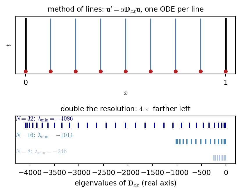
Heat Equation: Three Time Steppers
With \(r=\alpha k/h^2\) and \(\mathbf{A}=\alpha\mathbf{D}_{xx}\): \[ \begin{aligned} \text{FE: }&\ \mathbf{u}^{n+1}=(I+k\mathbf{A})\,\mathbf{u}^n\\ \text{BE: }&\ (I-k\mathbf{A})\,\mathbf{u}^{n+1}=\mathbf{u}^n\\ \text{CN: }&\ (I-\tfrac{k}{2}\mathbf{A})\,\mathbf{u}^{n+1}=(I+\tfrac{k}{2}\mathbf{A})\,\mathbf{u}^n \end{aligned} \]
| scheme | order in \((k,h)\) | stable for |
|---|---|---|
| forward Euler | \((1,2)\) | \(r\le\tfrac12\) |
| backward Euler | \((1,2)\) | any \(r\) |
| Crank-Nicolson | \((2,2)\) | any \(r\) |
Show code
def heat(N, k, T, scheme, f):
    h = 1 / N; x = np.arange(1, N) * h
    u, L, I = f(x), D_xx(N - 1, h), sp.identity(N - 1, format="csc")
    if scheme == "backward Euler":
        lu = splu(I - k * L)                           # factor once, reuse every step
    elif scheme == "Crank-Nicolson":
        lu = splu(I - k / 2 * L)
    for _ in range(int(round(T / k))):
        if scheme == "forward Euler":
            u = u + k * (L @ u)
        elif scheme == "backward Euler":
            u = lu.solve(u)
        else:
            u = lu.solve(u + k / 2 * (L @ u))
    return x, u

box = lambda x: ((x > 0.3) & (x < 0.6)).astype(float)
N, T = 50, 0.005; h = 1 / N; xf = np.linspace(0, 1, 400)
runs = [("forward Euler", 0.45), ("forward Euler", 0.55), ("backward Euler", 6.25), ("Crank-Nicolson", 6.25)]
fig, axs = plt.subplots(2, 2, figsize=(5.4, 3.6), sharex=True, sharey=True)
for ax, (name, r) in zip(axs.ravel(), runs):
    k = r * h**2
    x, u = heat(N, k, T, name, box)
    ax.plot(xf, heat_exact(box, xf, T), "k--", lw=1)
    ax.plot(x, np.clip(u, -1, 2), ".-", color=COL[name], lw=1, ms=3)
    ax.set_title(f"{name}, $r={r}$ ({int(round(T / k))} steps)", fontsize=8.5, color=COL[name])
    ax.set_ylim(-0.4, 1.1)
plt.tight_layout()
plt.show()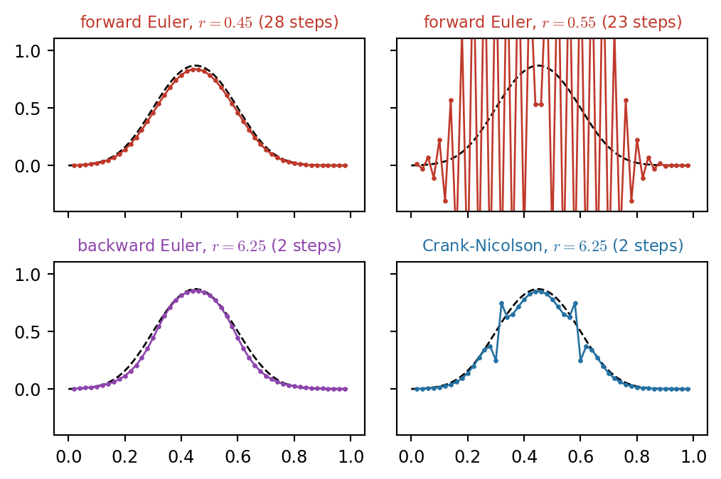
- Implicit: one tridiagonal solve per step, \(O(N)\). Factor once, reuse every step.
- CN keeps high modes with \(R\to-1\) (trapezoid): sharp data rings.
- In practice: start with BE for a few steps, then switch to CN.
Consistency + Stability = Convergence
- Consistent: the difference operators approach the derivatives as \(h,k\to0\) (Taylor series).
- Stable: errors stay bounded as steps accumulate.
- Convergent: the numerical solution approaches the true one as \(h,k\to0\). What we want.
For a well-posed linear problem:
consistency \(+\) stability \(\Longleftrightarrow\) convergence.
Practical check
When testing a scheme, always refine the grid and check the slope against the expected order.
Show code
f0 = lambda x: np.sin(np.pi * x) + 0.5 * np.sin(3 * np.pi * x)
exact = lambda x, t: (np.exp(-np.pi**2 * t) * np.sin(np.pi * x)
                      + 0.5 * np.exp(-9 * np.pi**2 * t) * np.sin(3 * np.pi * x))
T, Ns = 0.05, np.array([10, 20, 40, 80, 160])
tests = [("forward Euler", lambda h: 0.4 * h**2, "FE, $r=0.4$", "-"),
         ("backward Euler", lambda h: h / 4, "BE, $k=h/4$", "-"),
         ("Crank-Nicolson", lambda h: h / 4, "CN, $k=h/4$", "-"),
         ("forward Euler", lambda h: 0.6 * h**2, "FE, $r=0.6$ (unstable)", ":")]
fig, ax = plt.subplots(figsize=(4.8, 3.5))
for name, kf, label, ls in tests:
    err = []
    for N in Ns:
        k = T / max(1, round(T / kf(1 / N)))
        x, u = heat(N, k, T, name, f0)
        err.append(np.abs(u - exact(x, T)).max())
    col = "firebrick" if "unstable" in label else COL[name]
    ax.loglog(Ns, np.minimum(err, 1e3), "o" + ls, color=col, lw=1.5, ms=4, label=label)
ax.loglog(Ns, 0.5 / Ns**2, "k--", lw=0.8); ax.text(100, 0.5 / 100**2 * 0.4, "slope $-2$", fontsize=8)
ax.loglog(Ns, 0.6 / Ns, "k:", lw=0.8); ax.text(100, 0.6 / 100 * 1.4, "slope $-1$", fontsize=8)
ax.set_ylim(1e-6, 2e3); ax.set_xlabel("grid points $N$"); ax.set_ylabel("max error at $t=0.05$")
ax.set_title("measured convergence of the heat equation", fontsize=9)
ax.legend(fontsize=7.5, loc="upper left")
plt.tight_layout()
plt.show()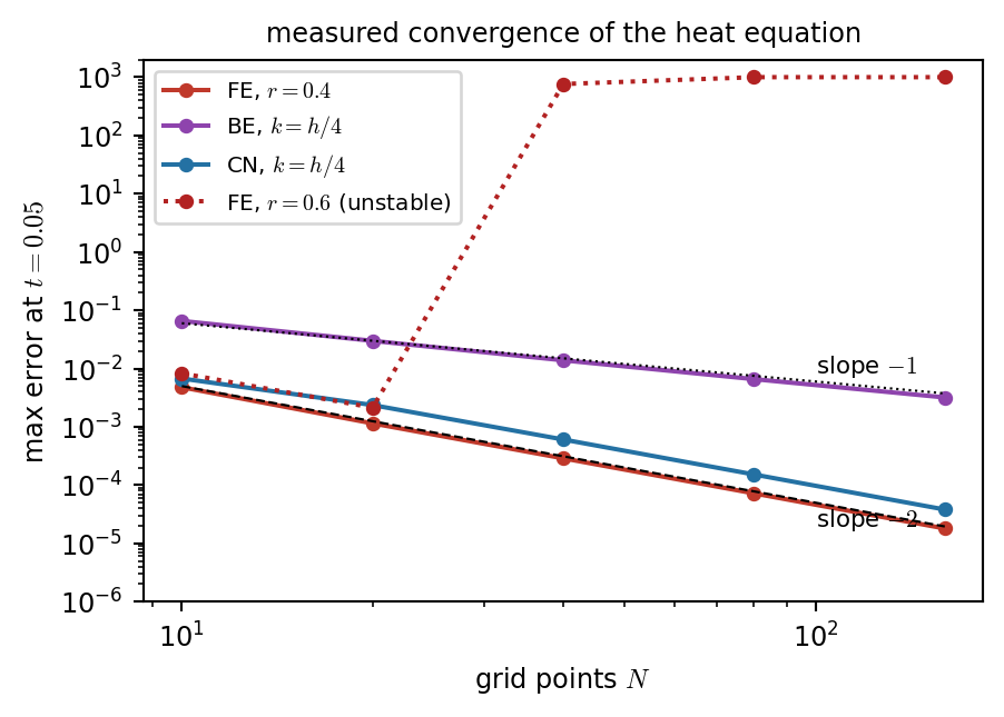
- Red line: consistent but unstable.
- It looks fine on coarse grids, then explodes as you refine. (definitely not convergent)
1D Wave Equation (1D WE)
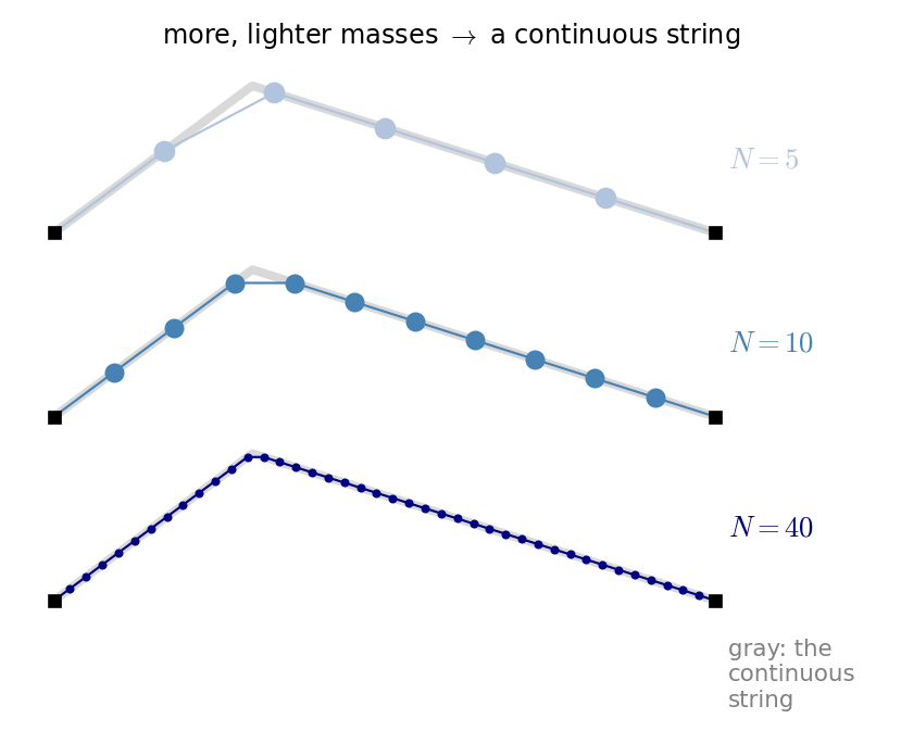
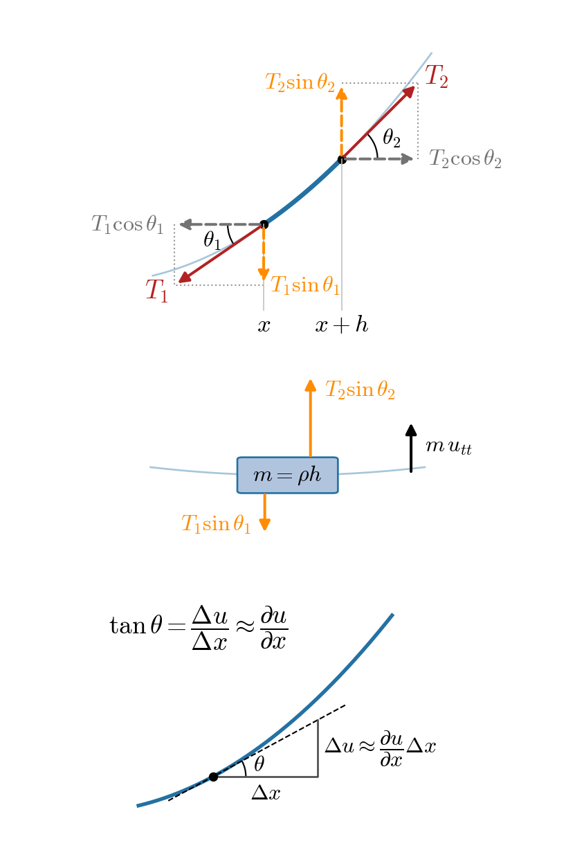
Horizontal tension equilibrium at a junction of two strings: \[ T_1\cos\theta_1 = T_2\cos\theta_2 \equiv T \tag{$\star$} \] Then the string’s vertical displacement \(u\) in \([x, x+h]\) satisfy \(m u_{tt} = T_2\sin\theta_2 - T_1\sin\theta_1\) by momentum conservation (Newton 2nd.) Divide both sides by \(T\) and use \((\star)\) to get \[\begin{aligned} \frac{\rho h}{T} u_{tt} &= \frac{T_2\sin\theta_2}{T_2\cos\theta_2} - \frac{T_1\sin\theta_1}{T_1\cos\theta_1} = \tan\theta_2 - \tan\theta_1 \\ &= \left(\frac{\partial u}{\partial x}\right)_{x+h} - \left(\frac{\partial u}{\partial x}\right)_x \end{aligned}\]
Take the limit \(h\to0\) to get \[ \frac{\rho}{T} u_{tt} = \frac{1}{h}\left[\left(\frac{\partial u}{\partial x}\right)_{x+h} - \left(\frac{\partial u}{\partial x}\right)_x\right] \stackrel{h\to 0}{\cong} \frac{\partial^2 u}{\partial x^2} \] Denote the wave speed \(c=\sqrt{T/\rho}\) then for \(x\in[0,L]\): \(\boxed{u_{tt}=c^2u_{xx}}\)
Or equivalently, using the velocity on the normalized domain \(x\in[0,1]\) with \(\gamma=c/L\): \(\boxed{u_{tt}=\gamma^2u_{xx}}\)
1D WE: General Solution
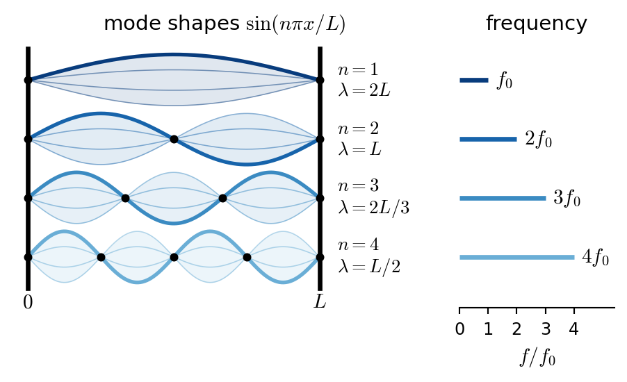
The solution of the 1D wave equation \(u_{tt} = c^2 u_{xx}\) is: \[\boxed{u(x, t) = A e^{j(\omega_n t \pm k_n x)}} \tag{$\star\star$}\] and the fundamental angular frequency \(\omega_0 = 2\pi f_0 = 2\pi \frac{c}{\lambda_0} = \frac{\pi c}{L}\), where \(\lambda_0 = 2L\) is the fundamental wavelength. The wave number \(k_n = n\frac{\omega_0}{c} = \frac{n\pi}{L}\) corresponds to the \(n\)-th harmonic (\(n,\omega_0\in\mathbb{R}\).)
- Plugging \((\star\star)\) into the wave equation gives \(\omega_n^2 = c^2 k_n^2\), which is also called as the dispersion relation of the 1D wave equation (will see more later.)
- Since \(\omega_n = c k_n\), the phase velocity \(v_p = \frac{\omega_n}{k_n} = c\) is independent of the frequency, which means that all frequencies travel at the same speed \(c\). This is called no dispersion.
Since \(k_n = n\frac{\omega_0}{c} = \frac{n\pi}{L}\), the \(n\)-th harmonic frequency is: \[\boxed{f_n = \frac{\omega_n}{2\pi} = \frac{n c}{2L} = n f_0}\]
Fundamental frequency and harmonics
- The fundamental frequency \(f_0 = \frac{c}{2L}\) is the lowest frequency of the string, and the higher harmonics are integer multiples of \(f_0\).
- Since \(c = \sqrt{T/\rho}\), \(f_0\) can be expressed using the tension \(T\) and density \(\rho\): \(\boxed{f_0 = \tfrac{1}{2L}\sqrt{\tfrac{T}{\rho}}}\)
1D WE: d’Alembert Solution
The wave equation \(u_{tt} = c^2 u_{xx}\) has a solution as superposition of two traveling waves: \[ u(x, t) = f(x + c t) + g(x - c t) \]
Proof
Introduce new coordinates \(\xi(x, t) = x - c t\) and \(\eta(x, t) = x + c t\) so that \(\tfrac{\partial\xi}{\partial x} = \tfrac{\partial\eta}{\partial x} = 1\), \(-\tfrac{\partial\xi}{\partial t} = \tfrac{\partial\eta}{\partial t} = c\).
Then chain rule + derivative of composite function gives \[\begin{aligned} u_x(x, t) &= \left(\frac{\partial}{\partial\xi}\frac{\partial\xi}{\partial x}\right) u = \frac{\partial}{\partial\xi} u \qquad &\Rightarrow\qquad u_{xx}(x,t) &= \left(\frac{\partial}{\partial\xi}\frac{\partial\xi}{\partial x}\right)\left[\frac{\partial}{\partial\xi} u(x, t)\right] = \frac{\partial^2}{\partial\xi^2} u(x, t) \\ u_t(x, t) &= \left(\frac{\partial}{\partial\eta}\frac{\partial\eta}{\partial t}\right) u = c\cdot\frac{\partial}{\partial\eta} u(x, t) \qquad &\Rightarrow\qquad u_{tt}(x, t) &= \left(\frac{\partial}{\partial\eta}\frac{\partial\eta}{\partial t}\right)\left[c\cdot\frac{\partial}{\partial\eta} u(x, t)\right] = c^2\cdot\frac{\partial^2}{\partial\eta^2} u(x, t) \end{aligned}\]
Injecting these into the wave equation gives
\[ 0 = c^2\frac{\partial^2}{\partial\eta^2} u(x, t) - c^2\frac{\partial^2}{\partial\xi^2} u(x, t) \qquad\iff\qquad \frac{\partial^2}{\partial\eta^2} u(x, t) = \frac{\partial^2}{\partial\xi^2} u(x, t)\tag{$*$} \]
Assume that \(u(x, t) = f(\eta) + g(\xi)\), so that \(\frac{\partial^2}{\partial\eta^2} u(x, t) = f''(\eta)\) and \(\frac{\partial^2}{\partial\xi^2} u(x, t) = g''(\xi)\). Then to examine if any form of \(f\) and \(g\) exists s.t. satisfy \((*)\), test: \(f(\eta) = \frac{c}{2}\eta^2 + B_1\eta + A_1\) and \(g(\xi) = \frac{c}{2}\xi^2 + B_2\xi + A_2\). Then \(f''(\eta) = g''(\xi) = c\) (satisfied.)
Above shows that there exists a solution \[\boxed{u(x, t) = f(\eta) + g(\xi) = \underbrace{f(x + c t)}_{\text{left-going}} + \underbrace{g(x - c t)}_{\text{right-going}}}\]
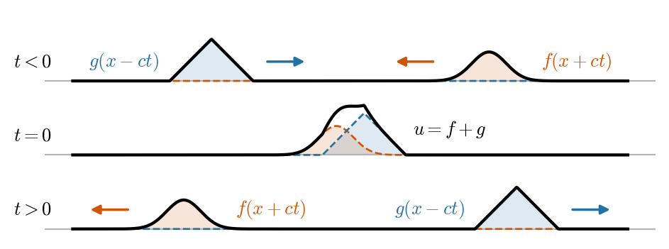
which is a superposition of two traveling waves, one moving to the left and the other moving to the right. cf. Traveling-wave solution
1D WE: Finite Difference Solution
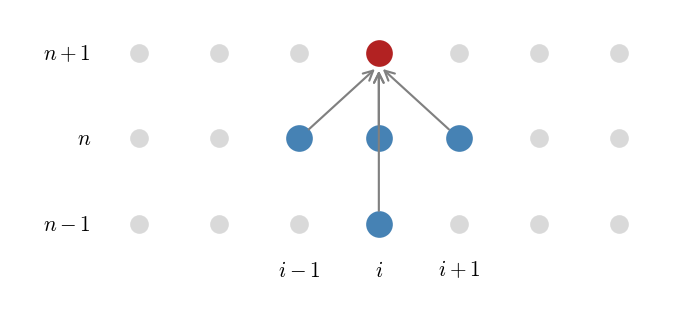
Finite difference with temporal \(k\) and spatial \(h\) step sizes: \[\begin{aligned} \delta_{tt}u &= c^2\,\delta_{xx}u \\ u_i^{(n+1)} - 2u_i^{(n)} + u_i^{(n-1)} &= \underbrace{\left(\frac{c k}{h}\right)^2}_{=: \lambda^2} \left(u_{i+1}^{(n)} - 2u_i^{(n)} + u_{i-1}^{(n)}\right) \end{aligned}\]
\[ u_i^{(n+1)} = 2u_i^{(n)} - u_i^{(n-1)} + \lambda^2 \left(u_{i+1}^{(n)} - 2u_i^{(n)} + u_{i-1}^{(n)}\right) \tag{$**$} \] Courant number \(\ \lambda=c k/h\): grid cells a wave crosses per step.
von Neumann stability analysis
To examine how each (spatial) Fourier mode behaves in time, assume a solution \(u_i^{(n)} = z^n e^{j\beta x_i} = z^n e^{j\cdot \beta \cdot i h}\) (where \(z^n = e^{j\omega t_k}\) and \(\beta\) is the grid wave number) and plug into \((**)\) to get the characteristic equation: \[z + 2\underbrace{(2\lambda^2\sin^2(\beta h/2) - 1 )}_{=:A} + z^{-1} = 0 \tag{$\circledast$}\] The roots are \(z_\pm = -A \pm \sqrt{A^2 - 1}\), and the scheme is stable if \(|z_\pm| \le 1\) for all \(\beta\).
- If \(|A| > 1\), then \(z_\pm\in\mathbb{R}\) and \(|z_\pm|^2 = (A\pm\sqrt{A^2 - 1})^2\) which is \(\beta\)-dependent (and can be greater than 1), so the scheme is unstable.
- If \(|A| \le 1\), then \(z_\pm\in\mathbb{C}\) and \(|z_\pm|^2 = A^2 + (1 - A^2) = 1\) for any \(\beta\), so the scheme is stable.
The CFL Condition
The von Neumann analysis gives the Courant-Friedrichs-Lewy (CFL) condition for stability: \[\begin{aligned} A\le 1 \ &\iff\ |2\lambda^2\sin^2(\beta h/2) - 1| \le 1 \\ &\iff\ \lambda^2\sin^2(\beta h/2) \le 1 \\ &\iff\ \lambda^2 \le 1 \ \iff\ \lambda = \frac{\gamma k}{h} \le 1 \end{aligned} \]
\[ \boxed{\lambda\le1}\quad\text{(Courant-Friedrichs-Lewy)} \]
- The numerical domain of dependence must contain the physical one (gray cone).
- Violations blow up at the spatial Nyquist wavelength \(2h\).
- At a fixed audio rate, CFL caps the grid: \(N\le f_s/\gamma\), i.e. \(2N\le2f_s/\gamma\) unknowns \(=\) the number of modes below Nyquist, times two. No resolution is wasted.
Show code
fig = plt.figure(figsize=(5.4, 3.8))
for j, (slope, title) in enumerate([(1.0, "$h=\\gamma k$: exact"), (1.5, "$h<\\gamma k$: unstable"), (0.7, "$h>\\gamma k$: stable")]):
    ax = fig.add_subplot(2, 3, j + 1)
    for n in range(4):
        ax.plot(range(-4, 5), [n] * 9, "o", color="0.85", ms=4)
    ax.fill([0, -3 * slope, 3 * slope], [3, 0, 0], color="0.6", alpha=0.35, lw=0)      # physical cone
    for n in range(4):                                                                  # numerical cone
        ax.plot(range(-(3 - n), 4 - n), [n] * (7 - 2 * n), "ko", ms=3.5)
    ax.plot([0, -3], [3, 0], "k--", lw=0.8); ax.plot([0, 3], [3, 0], "k--", lw=0.8)
    ax.set_xlim(-4.6, 4.6); ax.set_ylim(-0.4, 3.4); ax.axis("off")
    ax.set_title(title, fontsize=8.5)

def run_wave(N, lam, steps):
    x = np.linspace(0, 1, N + 1); u0 = 0.5 * (1 + np.cos(np.pi * np.clip((x - 0.5) / 0.1, -1, 1)))
    u = u0.copy(); up = u0.copy()
    for _ in range(steps):
        un = np.zeros_like(u)
        un[1:-1] = 2 * (1 - lam**2) * u[1:-1] + lam**2 * (u[2:] + u[:-2]) - up[1:-1]
        up, u = u, un
    return x, u
ax = fig.add_subplot(2, 1, 2)
for steps, col in [(0, "0.7"), (10, "steelblue"), (20, "darkorange"), (28, "firebrick")]:
    x, u = run_wave(80, 1.0125, steps)
    ax.plot(x, np.clip(u, -1.5, 1.5), color=col, lw=1.2, label=f"step {steps}")
ax.set_ylim(-1.5, 1.5); ax.legend(fontsize=7, ncol=4, loc="upper right"); ax.set_xlabel("$x$")
ax.set_title("$\\lambda=1.0125$: a 1% violation grows a zigzag of wavelength $2h$", fontsize=9)
plt.tight_layout()
plt.show()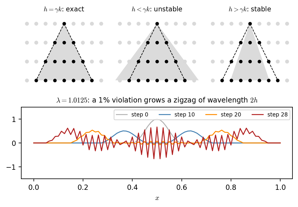
Numerical Dispersion: Why \(\lambda=1\) Is Special
Recall the characteristic equation \((\circledast)\) from the von Neumann analysis, substitute \(z = e^{j\omega k}\) and rearrange to get the numerical dispersion relation: \[\begin{aligned} &z + 2(2\lambda^2\sin^2(\beta h/2) - 1 ) + z^{-1} = 0 \\ \Rightarrow\quad &-4\sin^2(\omega k/2) + 4\lambda^2\sin^2(\beta h/2) = 0 \\ \Rightarrow\quad &\boxed{\sin\frac{\omega k}{2} = \pm\lambda\,\sin\frac{\beta h}{2}} \\ &\boxed{\omega = \pm\frac{2}{k}\arcsin\left(\lambda\,\sin\frac{\beta h}{2}\right)} \end{aligned}\]
Show code
fs, gamma = 44100, 440.0
k = 1 / fs
fig, axs = plt.subplot_mosaic([["vp", "x"], ["vg", "x"]], figsize=(5.6, 3.4), width_ratios=[1, 1.2])
for lam_t, col in [(1.0, "k"), (0.9, "steelblue"), (0.7, "darkorange"), (0.5, "firebrick")]:
    N = int(lam_t / (gamma * k)); h = 1 / N; lam = gamma * k / h
    beta = np.linspace(1e-6, 0.999 * np.pi / h, 400)       # up to the grid's highest wavenumber
    omega = 2 / k * np.arcsin(lam * np.sin(beta * h / 2))
    v_g = np.cos(beta * h / 2) / np.sqrt(1 - (lam * np.sin(beta * h / 2))**2)   # (d omega / d beta) / gamma
    f_kHz = omega / (2 * np.pi) / 1e3
    axs["vp"].plot(f_kHz, omega / (gamma * beta), color=col, lw=1.6)
    axs["vg"].plot(f_kHz, v_g, color=col, lw=1.6)
    xt, yt, ha = (f_kHz[-1] - 0.4, 0.9, "right") if lam_t == 1 else (f_kHz[-1] + 0.4, omega[-1] / (gamma * beta[-1]) - 0.02, "left")
    axs["vp"].text(xt, yt, f"$\\lambda={lam:.2f}$", color=col, fontsize=8, ha=ha, va="center")
    axs["vg"].text(f_kHz[-1] + (-0.2 if lam_t == 1 else 0.2), 0.05, f"$\\lambda={lam:.2f}$", color=col, fontsize=8,
                   rotation=90, va="bottom", ha="right" if lam_t == 1 else "left")
axs["vp"].set_ylabel("$v_\\phi/c$"); axs["vp"].set_ylim(0.6, 1.05)
axs["vp"].set_title("phase and group velocity", fontsize=9); axs["vp"].tick_params(labelbottom=False)
axs["vg"].set_ylabel("$v_g/c$"); axs["vg"].set_ylim(0, 1.1)
axs["vg"].set_xlabel("frequency (kHz)")
for a in ["vp", "vg"]: axs[a].set_xlim(0, 22.05)

def travel(lam, N=200, dist=0.5):                       # a narrow pulse, traveling right
    h = 1 / N; x = np.arange(N + 1) * h
    a = lambda s: np.exp(-((s - 0.2) / 0.012)**2)
    u0, u1 = a(x), a(x - lam * h)                       # exact first step of a right going wave
    for _ in range(int(round(dist / (lam * h))) - 1):
        un = np.zeros_like(u1)
        un[1:-1] = 2 * (1 - lam**2) * u1[1:-1] + lam**2 * (u1[2:] + u1[:-2]) - u0[1:-1]
        u0, u1 = u1, un
    return x, u1
for lam, col, off in [(1.0, "k", 0), (0.7, "darkorange", -1.2)]:
    x, u = travel(lam)
    axs["x"].plot(x, u + off, color=col, lw=1.2)
    axs["x"].text(0.42, off + 0.5, f"$\\lambda={lam}$", color=col, fontsize=9)
    axs["x"].annotate("", (0.81, off + 0.6), (0.73, off + 0.6),     # direction of travel
                    arrowprops=dict(arrowstyle="-|>", color=col, lw=1.3, mutation_scale=10))
axs["x"].axvline(0.7, color="0.8", ls="--", lw=0.8)
axs["x"].set_xlim(0.4, 0.85); axs["x"].set_yticks([]); axs["x"].set_xlabel("$x$")
axs["x"].set_title("a pulse after traveling 0.5: ripples trail", fontsize=9)
plt.tight_layout()
plt.show()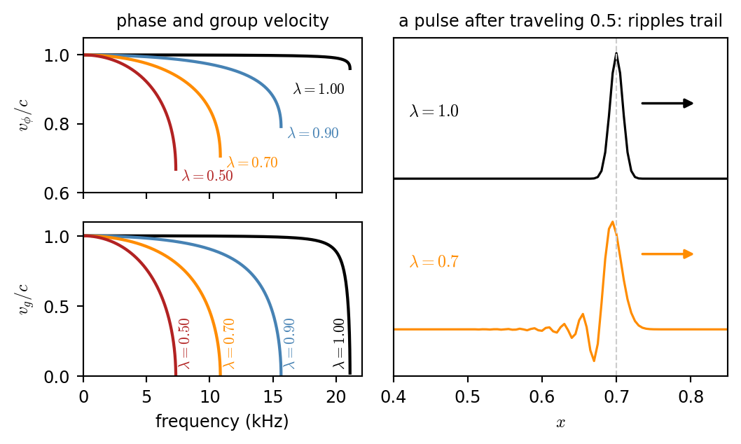
(cf. continuous case: \(\omega=\gamma\beta\), every wavelength at speed \(\gamma\)).
- \(\lambda=1\): \(\omega=\gamma\beta\) exactly. No numerical dispersion; the scheme is exact.
- \(\lambda<1\): short waves travel too slowly. High partials go flat, and the grid cannot carry anything above \[ f_{\max}=\frac{f_s}{\pi}\arcsin\lambda \qquad(f_{\max}<\frac{f_s}{2}) \]
- Audio rule: choose \(\lambda\) as close to \(1\) as stability allows.
Energy and Numerical Boundary Conditions
Multiply the scheme by \(\delta_{t\cdot}u\), sum over the grid, and sum by parts: \[ \mathfrak{h}^{n}=\underbrace{\tfrac12\lVert\delta_{t-}u^n\rVert^2}_{\text{kinetic}}+\underbrace{\tfrac{\gamma^2}{2}\bigl\langle\delta_{x+}u^n,\ \delta_{x+}u^{n-1}\bigr\rangle}_{\text{potential}} =\text{const} \]
- \(\mathfrak{h}\ge0\) only if \(\lambda\le1\): a second proof of CFL, the energy method. It still works for nonlinear schemes and awkward boundaries.
- Choose boundary conditions that make the boundary terms vanish:
- fixed: \(u_0=u_N=0\)
- free: virtual point \(u_{-1}=u_1\), and weight \(\tfrac12\) on the end points in \(\lVert\cdot\rVert\).
Show code
def wave_energy(N, lam, steps, bc):
    h = 1 / N; k = lam * h; x = np.arange(N + 1) * h      # gamma = 1
    u = pluck(x) if bc == "fixed" else np.exp(-((x - 0.3) / 0.1)**2)
    up, E = u.copy(), []
    w = np.ones(N + 1); w[[0, -1]] = 0.5                   # trapezoid weights for the free ends
    for _ in range(steps):
        un = np.zeros_like(u)
        un[1:-1] = 2 * (1 - lam**2) * u[1:-1] + lam**2 * (u[2:] + u[:-2]) - up[1:-1]
        if bc == "free":                                   # virtual points u_{-1} = u_1, u_{N+1} = u_{N-1}
            un[0] = 2 * (1 - lam**2) * u[0] + 2 * lam**2 * u[1] - up[0]
            un[-1] = 2 * (1 - lam**2) * u[-1] + 2 * lam**2 * u[-2] - up[-1]
        kinetic = 0.5 * h * np.sum(w * ((un - u) / k)**2)
        potential = 0.5 * h * np.sum((np.diff(un) / h) * (np.diff(u) / h))
        E.append(kinetic + potential)
        up, u = u, un
    E = np.array(E)
    return (E - E[0]) / E[0]

fig, ax = plt.subplots(figsize=(4.6, 3.4))
for bc, lam, col in [("fixed", 1.0, "steelblue"), ("fixed", 0.8, "lightsteelblue"),
                     ("free", 1.0, "darkorange"), ("free", 0.8, "navajowhite")]:
    ax.plot(wave_energy(100, lam, 2000, bc), ".", color=col, ms=1.5, label=f"{bc}, $\\lambda={lam}$")
ax.set_xlabel("time step"); ax.set_ylabel("relative energy change")
ax.set_title("energy is conserved to rounding error", fontsize=9)
ax.legend(fontsize=7.5, markerscale=6, loc="lower left"); ax.set_ylim(-4e-14, 4e-14)
plt.tight_layout()
plt.show()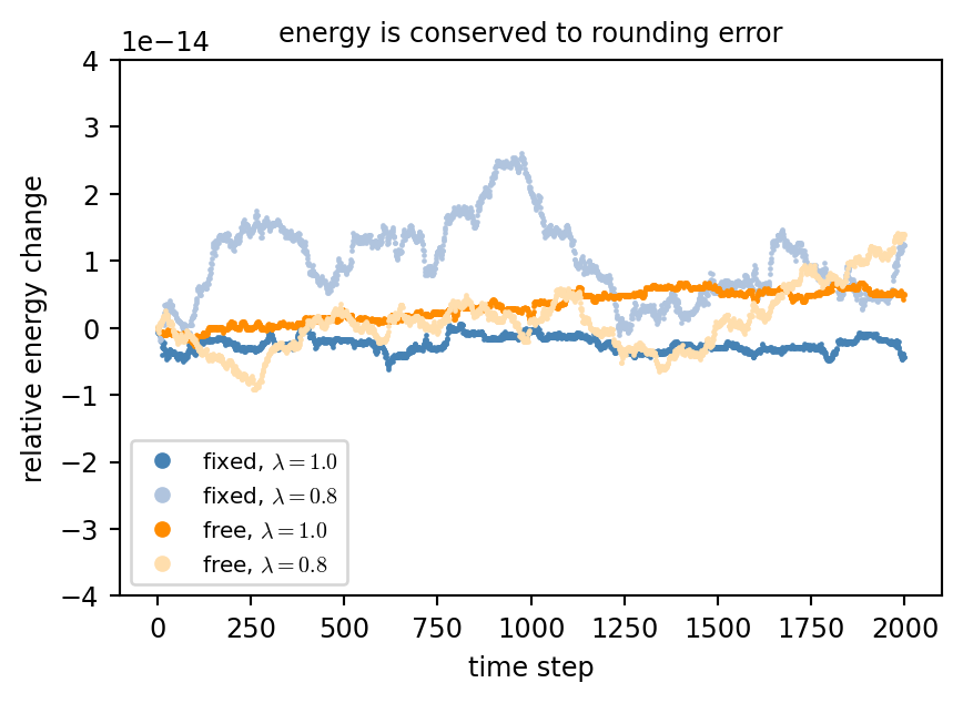
Loss: Letting the String Ring Down
\[ u_{tt}=\gamma^2u_{xx}-2\sigma_0u_t \qquad\Rightarrow\qquad \delta_{tt}u=\gamma^2\delta_{xx}u-2\sigma_0\,\delta_{t\cdot}u \] Still explicit: \(u_l^{n+1}\) appears only at its own point. \[ \begin{aligned} (1+\sigma_0k)\,u_l^{n+1}=\ &2(1-\lambda^2)\,u_l^n+\lambda^2\bigl(u_{l+1}^n+u_{l-1}^n\bigr)\\ &-(1-\sigma_0k)\,u_l^{n-1} \end{aligned} \]
- Set \(\sigma_0\) from the 60 dB decay time: \(\ T_{60}=3\ln10/\sigma_0\) (amplitude \(\propto e^{-\sigma_0t}\)).
- The energy can only decrease (passive), so stability is kept.
- But every partial decays at the same rate. A real pluck gets darker as it rings: high partials die first. Next class: frequency dependent loss.
Show code
fs, f0, T60 = 44100, 220.0, 1.5
k, gamma, sig0 = 1 / fs, 2 * f0, 3 * np.log(10) / T60
N = int(1 / (gamma * k)); h = 1 / N; lam = gamma * k / h
x = np.arange(N + 1) * h
u = pluck(x, 0.13); up = u.copy(); out, E = [], []
for n in range(int(2.0 * fs)):
    un = np.zeros_like(u)
    un[1:-1] = (2 * (1 - lam**2) * u[1:-1] + lam**2 * (u[2:] + u[:-2])
                - (1 - sig0 * k) * up[1:-1]) / (1 + sig0 * k)
    E.append(0.5 * h * np.sum(((un - u) / k)**2) + 0.5 * gamma**2 * h * np.sum(np.diff(un) / h * np.diff(u) / h))
    up, u = u, un; out.append(u[int(0.7 * N)])
out = np.array(out)
fig, axs = plt.subplots(2, 1, figsize=(4.8, 3.6), height_ratios=[1.6, 1])
win = 4096; hop = 1024
frames = np.array([np.abs(np.fft.rfft(out[i:i + win] * np.hanning(win))) for i in range(0, len(out) - win, hop)])
tf = (np.arange(len(frames)) * hop + win / 2) / fs
for p, col in zip(range(1, 7), plt.cm.viridis(np.linspace(0, 0.9, 6))):
    b = int(round(p * f0 * win / fs))
    axs[0].plot(tf, 20 * np.log10(frames[:, b - 2:b + 3].max(1) / frames.max()), color=col, lw=1.5, label=f"partial {p}")
axs[0].set_ylabel("dB"); axs[0].set_ylim(-90, 5); axs[0].legend(fontsize=6.5, ncol=3, loc="lower left")
axs[0].set_title(f"$T_{{60}}={T60}$ s: all partials decay in parallel", fontsize=9)
axs[1].plot(np.arange(len(E)) / fs, 10 * np.log10(np.array(E) / E[0]), color="k", lw=1.2)
axs[1].set_xlabel("time (s)"); axs[1].set_ylabel("energy (dB)")
plt.tight_layout()
plt.show()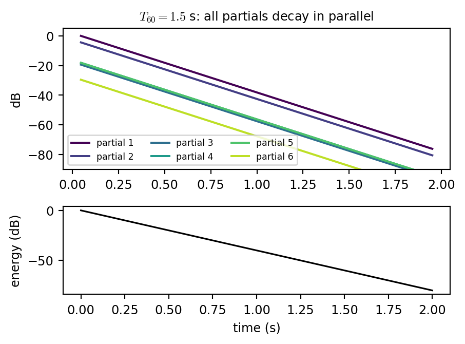
Digital Waveguides: The Exact Shortcut
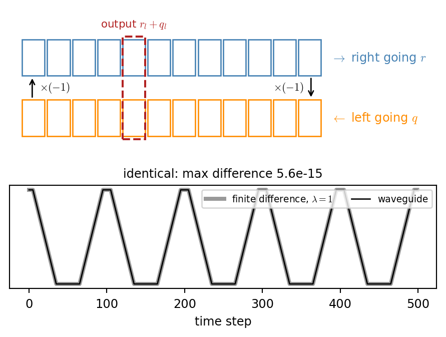
At \(\lambda=1\) the scheme is \(u_l^{n+1}=u_{l+1}^n+u_{l-1}^n-u_l^{n-1}\), and d’Alembert’s two traveling waves move exactly one cell per step:
- Store the right going wave \(r\) and the left going wave \(q\) in two delay lines.
- Each step: shift both, and reflect with a sign flip at the fixed ends.
- Output: \(u_l=r_l+q_l\).
| finite difference | waveguide | |
|---|---|---|
| cost per sample | \(O(N)\) | \(O(1)\) (circular buffers) |
| exact for | ideal string, \(\lambda=1\) | ideal string |
| stiffness, nonlinearity, 2D | natural | needs filter approximations |
Show code
N, steps, lo = 50, 500, 20
x = np.arange(N + 1) / N; u0 = pluck(x)
up, u = u0.copy(), u0.copy(); u[1:-1] = 0.5 * (u0[2:] + u0[:-2])   # lambda = 1 start
fd = [up[lo], u[lo]]
for _ in range(steps - 2):
    un = np.zeros_like(u); un[1:-1] = u[2:] + u[:-2] - up[1:-1]
    up, u = u, un; fd.append(u[lo])
r, q = u0 / 2, u0 / 2; dw = [u0[lo]]
for _ in range(steps - 1):
    r = np.r_[0, r[:-1]]; q = np.r_[q[1:], 0]
    r[0], q[-1] = -q[0], -r[-1]
    dw.append(r[lo] + q[lo])
fd, dw = np.array(fd), np.array(dw)

fig, axs = plt.subplots(2, 1, figsize=(4.8, 3.6), height_ratios=[1.4, 1])
ax = axs[0]
for y0, name, col, arrow in [(1, "right going $r$", "steelblue", "$\\rightarrow$"), (0, "left going $q$", "darkorange", "$\\leftarrow$")]:
    for i in range(12):
        ax.add_patch(plt.Rectangle((i, y0 - 0.3), 0.9, 0.6, fc="white", ec=col))
    ax.text(12.3, y0, f"{arrow} {name}", color=col, va="center", fontsize=9)
ax.annotate("", xy=(11.5, 0.3), xytext=(11.5, 0.7), arrowprops=dict(arrowstyle="->", color="k"))
ax.annotate("", xy=(0.4, 0.7), xytext=(0.4, 0.3), arrowprops=dict(arrowstyle="->", color="k"))
ax.text(11.2, 0.5, "$\\times(-1)$", ha="right", va="center", fontsize=8)
ax.text(0.7, 0.5, "$\\times(-1)$", ha="left", va="center", fontsize=8)
ax.add_patch(plt.Rectangle((4, -0.35), 0.9, 1.7, fc="none", ec="firebrick", lw=1.5, ls="--"))
ax.text(4.45, 1.5, "output $r_l+q_l$", color="firebrick", ha="center", fontsize=8)
ax.set_xlim(-0.5, 16.5); ax.set_ylim(-0.6, 1.8); ax.axis("off")
axs[1].plot(fd, color="0.6", lw=3, label="finite difference, $\\lambda=1$")
axs[1].plot(dw, color="k", lw=1, label="waveguide")
axs[1].set_xlabel("time step"); axs[1].set_yticks([])
axs[1].set_title(f"identical: max difference {np.abs(fd - dw).max():.1e}", fontsize=9)
axs[1].legend(fontsize=7, loc="upper right", ncol=2)
plt.tight_layout()
plt.show()