Ordinary Differential Equations II
Topics in Digital Heritage:
Numerical Methods for Digital Reconstruction
Fall 2026
Second Order Problems
Lots of physical problems are second order: Newton’s law \(M\mathbf{u}''=\mathbf{f}(\mathbf{u},\mathbf{u}')\). The unknown is position \(\mathbf{u}\), and the acceleration is a function of position and velocity.
Previously we converted second order problems into first order systems. Today we will treat them directly.
Today: Second Order Problems, Second Order Methods?
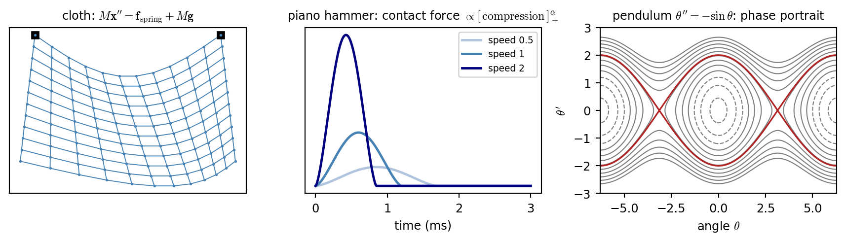
Second order problem: \(\ \mathbf{u}''=\mathbf{a}(\mathbf{u},\mathbf{u}')\) with \(\mathbf{u}(0)\), \(\mathbf{u}'(0)\). Do \(\mathbf{u}\) and \(\mathbf{u}'\) need the same accuracy? Can we run for thousands of periods without losing energy?
The Pendulum: A Second Order Problem
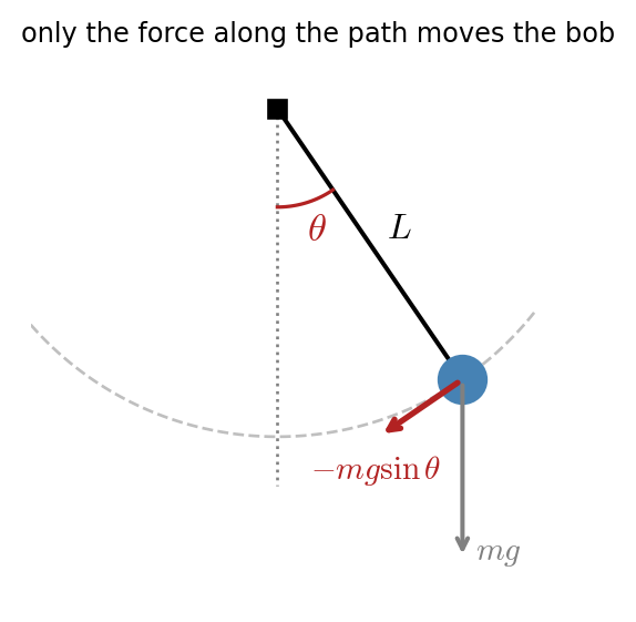
Newton along the arc (length \(L\theta\)): \[ mL\,\theta''=-mg\sin\theta \ \Rightarrow\ \theta''=-\sin\theta\quad(g/L=1) \]
- \(\mathbf{u}''=\mathbf{a}(\mathbf{u})\) with \(u=\theta\) and \(a(\theta)=-\sin\theta\). Give \(\theta(0)\) and \(\theta'(0)\).
- Small angles: \(\sin\theta\approx\theta\), the linear oscillator of last class. Large angles: nonlinear.
- No friction, so the energy \(H=\tfrac12\theta'^2-\cos\theta\) is conserved: our yardstick today.
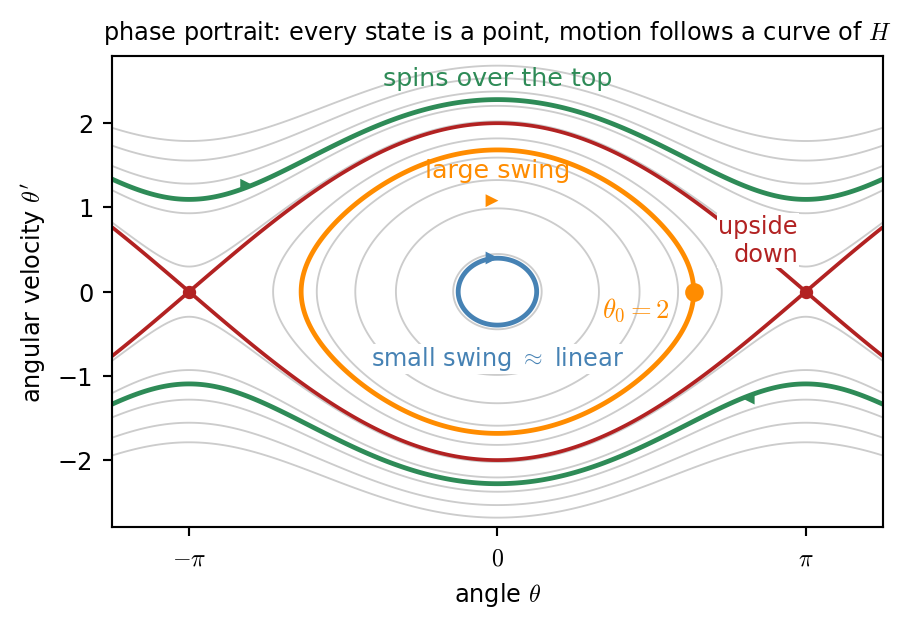
- A state \((\theta,\theta')\) is a point. As time passes it moves along a curve of constant \(H\).
- One loop is one back and forth swing. The orange loop (\(\theta_0=2\)) is today’s long run test.
- A method that gains energy drifts to outer curves, one that loses energy to inner curves.
Position and Velocity Deserve Different Care
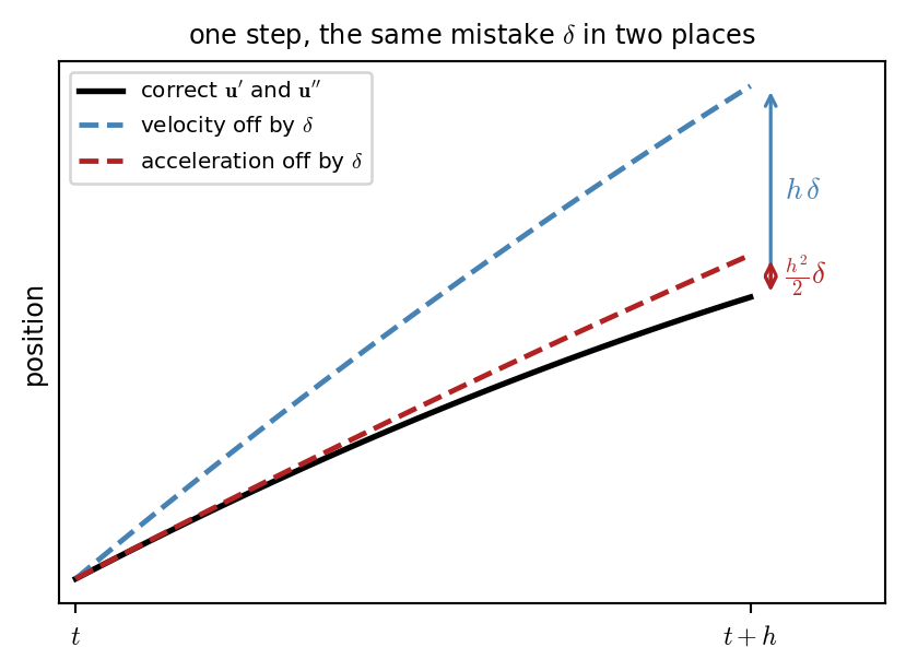
Predict the position one step ahead, as if throwing a ball: \[ \mathbf{u}(t+h)=\mathbf{u}+\underbrace{h}_{\text{weight}}\,\mathbf{u}'+\underbrace{\tfrac{h^2}{2}}_{\text{weight}}\,\mathbf{u}''+O(h^3) \]
- A mistake \(\delta\) in the velocity moves the prediction by \(h\,\delta\).
- The same mistake in the acceleration moves it only by \(\tfrac{h^2}{2}\delta\).
- For a second order accurate \(\mathbf{u}\), the error per step must be \(O(h^3)\). So an \(O(h^2)\) error in \(\mathbf{u}'\), or \(O(h)\) in \(\mathbf{u}''\), is good enough.
- If we care about position, velocity and acceleration can be computed less accurately, hence more cheaply.
- Solving \(\mathbf{y}'=F(\mathbf{y})\) with \(\mathbf{y}=(\mathbf{u},\mathbf{u}')\) treats them democratically and throws this freedom away.
Newmark: Blend the Accelerations at Both Ends
Notation. \(\mathbf{u}_k\approx\mathbf{u}(t_k)\), \(\mathbf{v}_k\approx\mathbf{u}'(t_k)\), and \(\mathbf{a}_k=\mathbf{a}(\mathbf{u}_k,\mathbf{v}_k)\) is the acceleration computed from the state at step \(k\) (Newton: \(\mathbf{a}=M^{-1}\mathbf{f}\); pendulum: \(a_k=-\sin\theta_k\)).
How \(\mathbf{a}\) varies inside the step is unknown, so blend the two ends: \[ \begin{aligned} \mathbf{u}_{k+1}&=\mathbf{u}_k+h\mathbf{v}_k+h^2\bigl[(\tfrac12-\beta)\,\mathbf{a}_k+\boldsymbol{\beta}\,\mathbf{a}_{k+1}\bigr]\\ \mathbf{v}_{k+1}&=\mathbf{v}_k+h\bigl[(1-\gamma)\,\mathbf{a}_k+\boldsymbol{\gamma}\,\mathbf{a}_{k+1}\bigr] \end{aligned} \]
- \(\mathbf{a}_{k+1}=\mathbf{a}(\mathbf{u}_{k+1},\dots)\) belongs to the future: it depends on the position we are computing.
- \(\beta\) and \(\gamma\) say how much to trust that future value, in the position and in the velocity.
- \(\beta>0\): \(\mathbf{u}_{k+1}\) and \(\mathbf{a}_{k+1}\) need each other, so each step solves an equation (implicit). \(\beta=0\): the loop is cut, so the step is explicit.
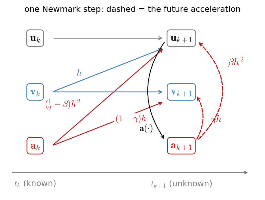
The loop \(\mathbf{u}_{k+1}\to\mathbf{a}_{k+1}\to\mathbf{u}_{k+1}\) is what makes the step implicit. It disappears when \(\beta=0\).
Newmark: Choosing \(\beta\) and \(\gamma\)
| \((\beta,\gamma)\) | name | type | stability |
|---|---|---|---|
| \((0,\tfrac12)\) | central difference | explicit | \(\omega h<2\) |
| \((\tfrac14,\tfrac12)\) | average acceleration (trapezoid) | implicit | any \(h\), keeps amplitude |
| \((\beta,\gamma>\tfrac12)\) | damped variant | implicit | any \(h\) if \(2\beta\ge\gamma\), damps high \(\omega\) |
- \(\beta\) sets the cost: \(\beta=0\) is explicit.
- \(\gamma\) sets the damping: second order only for \(\gamma=\tfrac12\). \(\gamma>\tfrac12\) leans toward backward Euler and damps (used to clean mesh noise in finite elements).
- Unconditionally stable when \(2\beta\ge\gamma\ge\tfrac12\).
- The cheapest member, \((0,\tfrac12)\), is our old friend: eliminating \(\mathbf{v}\) gives \(\dfrac{\mathbf{u}_{k+1}-2\mathbf{u}_k+\mathbf{u}_{k-1}}{h^2}=\mathbf{a}(\mathbf{u}_k)\), the \(\delta_{tt}\) scheme of class 10.
Show code
def newmark_matrix(x, beta, gamma):                # one step on u'' = -u with h = x, state (u, v)
    A = np.empty((2, 2))
    for j, (u, v) in enumerate([(1.0, 0.0), (0.0, 1.0)]):
        a = -u
        u_p = u + x * v + (0.5 - beta) * x**2 * a
        v_p = v + (1 - gamma) * x * a
        a = -u_p / (1 + beta * x**2)
        A[:, j] = [u_p + beta * x**2 * a, v_p + gamma * x * a]
    return A

wh = np.linspace(0.01, 4, 400)
fig, ax = plt.subplots(figsize=(4.4, 2.7))
for (b, g), col, ls, lab in [((0.25, 0.5), COL["trapezoid"], "-", "$(\\frac{1}{4},\\frac{1}{2})$ average acceleration"),
                             ((0, 0.5), COL["leapfrog"], "--", "$(0,\\frac{1}{2})$ central difference"),
                             ((0.3025, 0.6), COL["backward Euler"], "-", "$(0.30,0.6)$ damped")]:
    gain = [max(abs(np.linalg.eigvals(newmark_matrix(x, b, g)))) for x in wh]
    ax.plot(wh, gain, color=col, ls=ls, lw=1.8, label=lab)
ax.axhline(1, color="gray", lw=0.8, ls=":")
ax.set_ylim(0.8, 1.6); ax.set_xlabel("$\\omega h$"); ax.set_ylabel("amplitude gain per step")
ax.set_title("$u''=-\\omega^2u$: above 1 blows up, below 1 damps", fontsize=9)
ax.legend(fontsize=7.5, loc="upper left")
plt.tight_layout()
plt.show()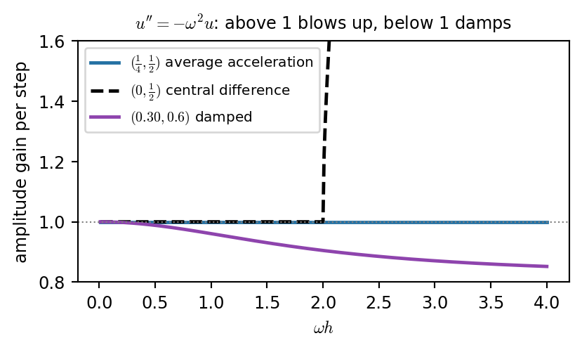
Code: one Newmark step for \(M\mathbf{u}''=-K\mathbf{u}\)
Leapfrog: Position and Velocity Take Turns
Speed measured between two mile markers is the speed halfway between them. So keep velocities at half steps, and both updates become centered differences: \[ \mathbf{u}_{k+1}=\mathbf{u}_k+h\,\mathbf{v}_{k+1/2},\qquad \mathbf{v}_{k+3/2}=\mathbf{v}_{k+1/2}+h\,\mathbf{a}(\mathbf{u}_{k+1}) \]
- Explicit when \(\mathbf{a}\) depends on \(\mathbf{u}\) only, with one evaluation of \(\mathbf{a}\) per step: the cost of forward Euler, but second order.
- Eliminating \(\mathbf{v}\) gives \(\delta_{tt}\mathbf{u}=\mathbf{a}(\mathbf{u})\) again: class 10’s scheme = Newmark central difference = leapfrog, three names for one method.
Störmer-Verlet: kick, drift, kick
Split the velocity update into two half kicks, so \(\mathbf{u}\) and \(\mathbf{v}\) are reported at the same time.
The first half kick also starts the scheme from \(\mathbf{v}(0)\).
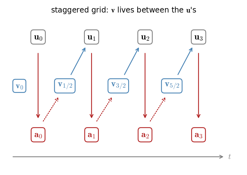
Every arrow points forward in time: no loop, nothing to solve. Same idea as class 10: differences live at the midpoint.
What Is a Symplectic Integrator?
Show code
accel = lambda th: -np.sin(th)                     # pendulum theta'' = -sin(theta)
energy = lambda th, w: 0.5 * w**2 - np.cos(th)

def forward_euler(u, v, h):
    return u + h * v, v + h * accel(u)

def leapfrog(u, v, h):                             # kick, drift, kick
    v = v + h / 2 * accel(u)
    u = u + h * v
    return u, v + h / 2 * accel(u)

def backward_euler(u, v, h):                       # Newton on u1 = u + h v - h^2 sin(u1)
    x = u + h * v
    for _ in range(30):
        x = x - (x - u - h * v + h**2 * np.sin(x)) / (1 + h**2 * np.cos(x))
    return x, v + h * accel(x)

def area(u, v):                                    # shoelace formula
    return 0.5 * abs(np.dot(u, np.roll(v, -1)) - np.dot(v, np.roll(u, -1)))

s = np.linspace(0, 2 * np.pi, 400, endpoint=False)
u0, v0 = 1.2 + 0.3 * np.cos(s), 0.3 * np.sin(s)    # a disk of initial states
h, n = 0.3, 12
TH, W = np.meshgrid(np.linspace(-2.7, 2.7, 300), np.linspace(-1.7, 1.7, 300))
fig, axs = plt.subplots(1, 3, figsize=(8, 4), sharey=True)
for ax, (name, step) in zip(axs, [("forward Euler", forward_euler), ("leapfrog", leapfrog), ("backward Euler", backward_euler)]):
    u, v = u0.copy(), v0.copy()
    for _ in range(n):
        u, v = step(u, v, h)                       # every state in the cloud takes a step
    ratio = area(u, v) / area(u0, v0)
    ue, ve = u0.copy(), v0.copy()                  # reference: tiny steps
    for _ in range(30 * n):
        ue, ve = leapfrog(ue, ve, h / 30)
    ax.contour(TH, W, energy(TH, W), levels=np.linspace(-0.9, 2.0, 9), colors="0.85", linewidths=0.6, linestyles="solid")
    ax.fill(u0, v0, color="0.6", alpha=0.6, lw=0)
    ax.plot(ue, ve, color="0.4", ls="--", lw=1)
    ax.fill(u, v, color=COL[name], alpha=0.35, lw=0); ax.plot(u, v, color=COL[name], lw=1.2)
    ax.set_title(f"{name}\n{n} steps: area $\\times${ratio:.2f}", fontsize=8.5, color=COL[name])
    ax.set_xlabel("$\\theta$"); ax.set_aspect("equal"); ax.set_xlim(-2.7, 2.7); ax.set_ylim(-1.7, 1.7)
axs[0].set_ylabel("$\\theta'$")
plt.tight_layout()
plt.show()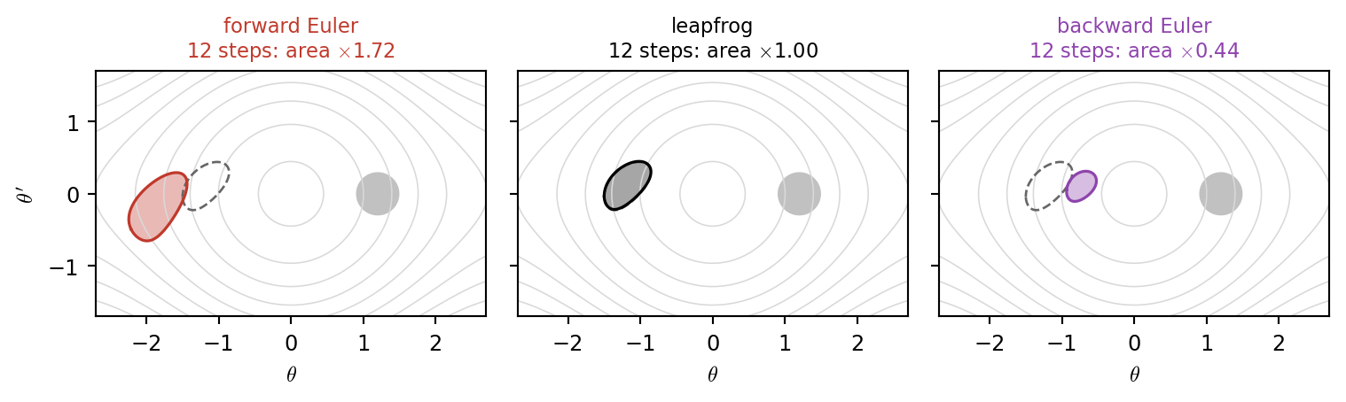
- A state \((\mathbf{u},\mathbf{u}')\) is a point in phase space, and one step maps points to points. Follow a whole cloud of nearby states (gray disk; dashed: exact).
- Frictionless physics deforms the cloud but keeps its area (Liouville’s theorem).
- A symplectic integrator is a step map that also keeps this area. With many degrees of freedom, it keeps the sum of the areas in each \((u_i,u_i')\) plane.
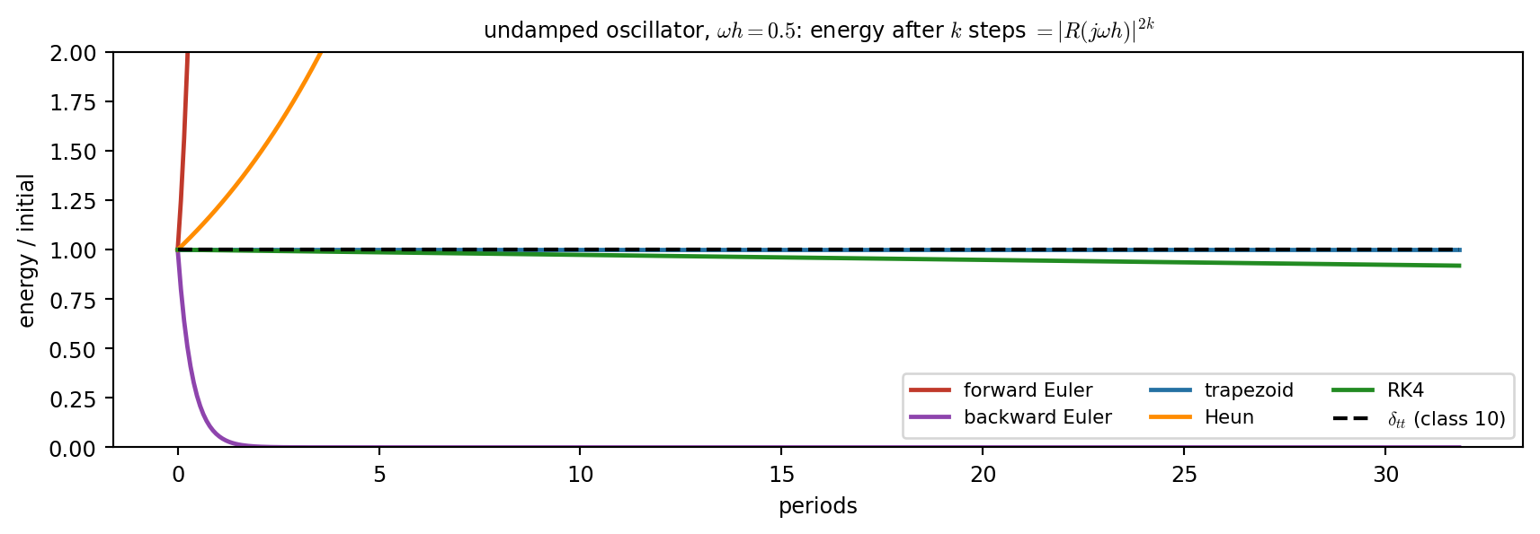
- On \(u''=-\omega^2u\) the area factor per step is the determinant of the step matrix: forward Euler \(1+\omega^2h^2\), backward Euler \(\frac{1}{1+\omega^2h^2}\), RK4 slightly below \(1\), and exactly \(1\) for leapfrog, symplectic Euler, and average acceleration Newmark.
- Growing area pushes the cloud to higher energy, shrinking to lower. A symplectic step exactly conserves a modified energy \(\widetilde{H}=H+O(h^2)\), so the true energy oscillates but cannot drift.
Thousands of Periods Later: Who Drifts?
Show code
accel = lambda th: -np.sin(th)                     # pendulum theta'' = -sin(theta)
energy = lambda th, w: 0.5 * w**2 - np.cos(th)

def leapfrog(u, v, a, h):                          # kick, drift, kick: one accel per step
    v = v + h / 2 * a
    u = u + h * v
    a = accel(u)
    return u, v + h / 2 * a, a

def symplectic_euler(u, v, a, h):
    v = v + h * a
    u = u + h * v
    return u, v, accel(u)

def newmark(u, v, a, h, beta=0.25, gamma=0.5):     # Newton for the new position
    u_p = u + h * v + (0.5 - beta) * h**2 * a
    v_p = v + (1 - gamma) * h * a
    x = u_p
    for _ in range(20):
        dx = (x - u_p - beta * h**2 * accel(x)) / (1 + beta * h**2 * np.cos(x))
        x -= dx
        if abs(dx) < 1e-15:
            break
    a = accel(x)
    return x, v_p + gamma * h * a, a

def rk4(u, v, a, h):                               # classical RK4 on y = (u, v)
    F = lambda y: np.array([y[1], accel(y[0])])
    y = np.array([u, v])
    k1 = F(y); k2 = F(y + h / 2 * k1); k3 = F(y + h / 2 * k2); k4 = F(y + h * k3)
    u, v = y + h / 6 * (k1 + 2 * k2 + 2 * k3 + k4)
    return u, v, accel(u)

th0, h, T = 2.0, 0.3, 3000.0
E0 = energy(th0, 0.0)
NEWMARK, DAMPED = "Newmark $(\\frac{1}{4},\\frac{1}{2})$", "Newmark $(0.30,0.6)$"
COL[NEWMARK], COL[DAMPED] = COL["trapezoid"], COL["backward Euler"]
steps = {"RK4": rk4,
         DAMPED: lambda u, v, a, h: newmark(u, v, a, h, 0.3025, 0.6),
         "symplectic Euler": symplectic_euler,
         NEWMARK: newmark,
         "leapfrog": leapfrog}

def run(step, h, n, back=False):   # energy history, or the distance from the start after n steps forward and n back
    u, v, a = th0, 0.0, accel(th0)
    E = np.empty(n)
    for i in range(n):
        u, v, a = step(u, v, a, h)
        E[i] = energy(u, v)
    if not back:
        return E
    for _ in range(n):
        u, v, a = step(u, v, a, -h)
    return max(abs(u - th0) + abs(v), 1e-17)

fig, axs = plt.subplots(1, 2, figsize=(9, 2.8), width_ratios=[1.7, 1])
blk = 100
def curve(E, hh, blk, col, label, ls="-", nudge=1.0):         # worst energy error in each block of steps, labeled at the end
    err = np.abs(E - E0).reshape(-1, blk).max(1)
    axs[0].semilogy(hh * blk * np.arange(1, len(err) + 1), err, color=col, lw=1.6, ls=ls)
    axs[0].text(T * 1.02, err[-1] * nudge, label, color=col, fontsize=7, va="center")
nudge = {"leapfrog": 1.35, NEWMARK: 0.75}
for name, step in steps.items():
    curve(run(step, h, int(T / h)), h, blk, COL[name], name, nudge=nudge.get(name, 1.0))
curve(run(steps["leapfrog"], h / 4, int(4 * T / h)), h / 4, 4 * blk, "gray", f"leapfrog, $h={h / 4}$\n(same cost as RK4)", ls="--")
axs[0].set_xlim(0, 1.45 * T); axs[0].set_ylim(5e-4, 4)
axs[0].set_xlabel("$t$"); axs[0].set_ylabel("|energy error|")
axs[0].set_title(f"pendulum, $\\theta_0={th0}$, $h={h}$, about {T / 8.6:.0f} periods", fontsize=9)

names = ["leapfrog", NEWMARK, "RK4", "symplectic Euler", DAMPED]
errs = [run(steps[nm], h, 1000, back=True) for nm in names]
axs[1].barh(range(len(names)), errs, color=[COL[nm] for nm in names])
axs[1].set_yticks(range(len(names))); axs[1].set_yticklabels(names, fontsize=7.5); axs[1].invert_yaxis()
axs[1].set_xscale("log"); axs[1].set_xlabel("distance from the start")
axs[1].set_title("1000 steps forward, then 1000 with $-h$", fontsize=9)
plt.tight_layout()
plt.show()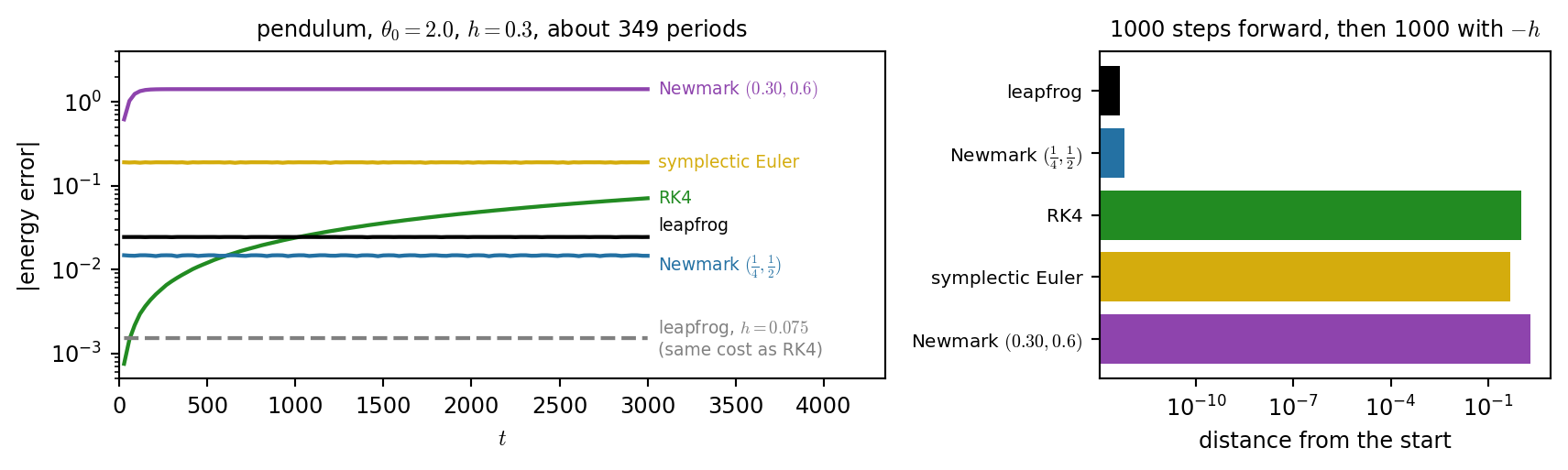
- RK4 starts most accurate but keeps losing energy: it is not symplectic, so the area shrinks a little every step (drift).
- Leapfrog, symplectic Euler, Newmark \((\frac14,\frac12)\): the error oscillates but stays flat for 350 periods.
- Damped Newmark (\(\gamma>\frac12\)) kills the swing: damping meant for mesh noise is poison for a ringing oscillator.
- At equal cost (4 leapfrog steps per RK4 step), leapfrog wins from start to end.
- Time reversibility: leapfrog and Newmark \((\frac14,\frac12)\) are symmetric, so stepping with \(-h\) exactly undoes \(+h\), as physics does. The others do not return.
- Higher order does not mean better in the long run. RK4 for a few periods. For thousands, a structure preserving method: leapfrog if explicit is enough, average acceleration if the step must be unconditionally stable.
Energy Is Kept, but Is the Pitch Right?
Leapfrog on \(u''=-\omega^2u\) is a two step recursion: \[ u_{k+1}=\bigl(2-\omega^2h^2\bigr)\,u_k-u_{k-1} \ \Rightarrow\ \sin\tfrac{\widetilde{\omega} h}{2}=\tfrac{\omega h}{2} \]
- The energy is kept, but the oscillator rings at a slightly wrong frequency \(\widetilde{\omega}\ne\omega\).
- Leapfrog plays sharp. Average acceleration plays flat: \(\tan\tfrac{\widetilde{\omega} h}{2}=\tfrac{\omega h}{2}\). Both errors are \(O(\omega^2h^2)\).
- For high partials at audio rates the error exceeds a semitone: audible.
- Energy and pitch are separate questions. Symplectic methods fix the drift, not the phase error.
- Fix for a linear oscillator: \(2-\omega^2h^2\) is just the start of the Taylor series of \(2\cos(\omega h)\). Use the whole thing, \(u_{k+1}=2\cos(\omega h)\,u_k-u_{k-1}\), and the pitch is exact for any \(h\).
- Coupled linear systems: split into modes first (modal method, last class). Large or nonlinear systems cannot be split, so we are back to time stepping: the rest of today.
Show code
wh = np.linspace(0.01, 1.99, 300)
lf = lambda x: 2 * np.arcsin(x / 2) / x             # leapfrog: sin(w~h/2) = wh/2
tr = lambda x: 2 * np.arctan(x / 2) / x             # average acceleration: tan(w~h/2) = wh/2
x8 = 2 * np.pi * 8000 / 44100                       # an 8 kHz partial at 44.1 kHz
fig, ax = plt.subplots(figsize=(4.4, 3.4))
ax.axhspan(2**(-1 / 12), 2**(1 / 12), color="0.92", lw=0, label="within a semitone")
ax.plot(wh, lf(wh), color=COL["leapfrog"], lw=1.8, label="leapfrog = central difference")
ax.plot(wh, tr(wh), color=COL["trapezoid"], lw=1.8, label="average acceleration")
ax.axhline(1, color="gray", ls="--", lw=1, label="exact")
ax.axvline(x8, color="gray", lw=0.8, ls=":")
for f, col, dy in [(lf, COL["leapfrog"], 0.07), (tr, COL["trapezoid"], -0.07)]:
    ax.plot(x8, f(x8), "o", color=col, ms=5)
    ax.text(x8 - 0.05, f(x8) + dy, f"{100 * (f(x8) - 1):+.1f}%", color=col, ha="right", va="center", fontsize=8)
ax.text(x8, 0.72, " 8 kHz at 44.1 kHz", color="gray", fontsize=7.5)
ax.set_xlim(0, 2); ax.set_ylim(0.7, 1.6)
ax.set_xlabel("$\\omega h$"); ax.set_ylabel("$\\tilde\\omega/\\omega$")
ax.set_title("numerical pitch over true pitch", fontsize=9)
ax.legend(fontsize=7, loc="upper left")
plt.tight_layout()
plt.show()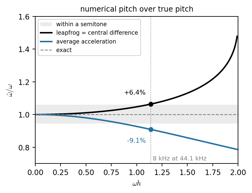
Chains of Masses: The Stiffest Spring Sets the Pace
\(N\) masses in a row, springs between neighbors: \[ m\,u_l''=K_s\,(u_{l+1}-u_l)-K_s\,(u_l-u_{l-1}) \ \Rightarrow\ M\mathbf{u}''=-K\mathbf{u} \] \(K\) is tridiagonal.
Explicit: \(\ \mathbf{u}^{n+1}=(2I-k^2M^{-1}K)\,\mathbf{u}^n-\mathbf{u}^{n-1}\), \(O(N)\) per step.
Stable when every mode satisfies \(\omega_pk<2\): \[ k\le\frac{2}{\sqrt{\lambda_{\max}(M^{-1}K)}} \] The stiffest, lightest part sets the step.
The price of resolution
- Finer rope \(\Rightarrow\) lighter masses, stiffer springs \(\Rightarrow\) \(k_{\max}\propto1/N\). Double the resolution: half the step, \(4\times\) the cost. (Preview of the CFL condition.)
- Implicit (Newmark \(\beta>0\), backward Euler): no limit, but a sparse SPD solve per step (CG, class 6).
Show code
def spring(ax, p, q, coils=6, amp=0.04, **kw):
    """Zigzag spring from point p to point q."""
    p, q = np.asarray(p, float), np.asarray(q, float)
    d = q - p; L = np.hypot(*d); t = d / L; n = np.array([-t[1], t[0]])
    s = np.r_[0, 0.15, np.linspace(0.15, 0.85, 2 * coils + 1)[1:-1], 0.85, 1]
    w = np.r_[0, 0, amp * (-1) ** np.arange(2 * coils - 1), 0, 0]
    pts = p + np.outer(s * L, t) + np.outer(w, n)
    ax.plot(pts[:, 0], pts[:, 1], **{"color": "0.6", "lw": 1, **kw})

def arrow(ax, p, d, col, lw=1.6, ls="-"):
    ax.annotate("", (p[0] + d[0], p[1] + d[1]), p, zorder=5,
                arrowprops=dict(arrowstyle="-|>", color=col, lw=lw, ls=ls, mutation_scale=9, shrinkA=0, shrinkB=0))

def pull(ax, i, j, col):
    """Spring force on mass i from its neighbor j: along the spring, split into horizontal and vertical."""
    d = np.array([x[j] - x[i], u[j] - u[i]]) * a        # tension along the spring
    p = (x[i], u[i])
    arrow(ax, p, d, "0.35", lw=1)                       # tension (along spring)
    arrow(ax, p, (d[0], 0), "0.35", lw=0.9, ls=(0, (2, 2)))  # horizontal part
    arrow(ax, (x[i] + d[0], u[i]), (0, d[1]), col, lw=1.8)   # vertical part: K_s (u_j - u_i)

x = np.array([-0.6, 0, 1, 2, 2.6])         # masses l-1, l, l+1 (and the chain beyond)
u = np.array([-0.15, 0.1, 1.0, 0.6, 0.35])
a = 0.42                                   # arrow length per unit (u_j - u_i)
c_left, c_right = COL["trapezoid"], "#d68910"

fig, ax = plt.subplots(figsize=(4.3, 2.4))
ax.axhline(0, color="0.75", lw=0.8, ls="--", zorder=0)
for i in (1, 2, 3):
    ax.axvline(x[i], color="0.88", lw=2.5, zorder=0)    # vertical rail: masses move only up and down
spring(ax, (x[0], u[0]), (x[1], u[1]), alpha=0.5)
spring(ax, (x[3], u[3]), (x[4], u[4]), alpha=0.5)
spring(ax, (x[1], u[1]), (x[2], u[2]), color=c_left, alpha=0.5)
spring(ax, (x[2], u[2]), (x[3], u[3]), color=c_right, alpha=0.5)
ax.plot(x[[1, 3]], u[[1, 3]], "o", ms=9, color="0.55", zorder=3)
ax.plot(x[2], u[2], "o", ms=10, color="firebrick", zorder=4)

pull(ax, 2, 1, c_left); pull(ax, 1, 2, c_left)        # left spring: equal and opposite
pull(ax, 2, 3, c_right); pull(ax, 3, 2, c_right)      # right spring: equal and opposite
net = a * (u[1] + u[3] - 2 * u[2])
arrow(ax, (x[2], u[2]), (0, net), "firebrick", lw=2.2)
fl, fr = a * (u[1] - u[2]), a * (u[3] - u[2])        # tip to tail: blue then orange = net
arrow(ax, (x[2] - 0.05, u[2]), (0, fl), c_left, lw=1.8)
arrow(ax, (x[2] - 0.05, u[2] + fl), (0, fr), c_right, lw=1.8)

ax.text(x[2] - a - 0.05, u[2] - 0.2, r"$-K_s(u_l-u_{l-1})$", color=c_left, ha="right", va="center", fontsize=8)
ax.text(x[2] + a + 0.05, u[2] - 0.05, r"$K_s(u_{l+1}-u_l)$", color=c_right, ha="left", va="center", fontsize=8)
ax.text(x[2] + 0.05, u[2] + net, "net", color="firebrick", ha="left", va="top", fontsize=8)
ax.text(x[2] - 0.22, u[2] + 0.04, "horizontal parts cancel", color="0.35", ha="center", va="bottom", fontsize=7)
for i, lab in [(1, "$m_{l-1}$"), (2, "$m_l$"), (3, "$m_{l+1}$")]:
    ax.text(x[i], -0.2, lab, ha="center", va="top", fontsize=8)
ax.plot([x[2] + 0.08] * 2, [0, u[2]], color="firebrick", lw=0.8, ls=":")
ax.text(x[2] + 0.1, 0.15, "$u_l$", color="firebrick", ha="left", fontsize=9)
ax.set_xlim(-0.6, 2.6); ax.set_ylim(-0.4, 1.25)
ax.axis("off")
plt.tight_layout()
plt.show()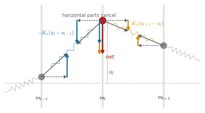
Application: Cloth as a Mass-Spring Network
Grid of masses; structural and shear springs; two corners pinned; gravity.
Spring from \(i\) to \(j\), rest length \(L\): \(\ \mathbf{f}_i=K_s\,(\lVert\mathbf{d}\rVert-L)\,\dfrac{\mathbf{d}}{\lVert\mathbf{d}\rVert},\ \ \mathbf{d}=\mathbf{x}_j-\mathbf{x}_i\)
- Explicit (symplectic Euler): \(\mathbf{v}\mathrel{+}=hM^{-1}\mathbf{f}(\mathbf{x})\), \(\ \mathbf{x}\mathrel{+}=h\mathbf{v}\).
- Implicit (backward Euler, one Newton step): \[\Bigl(M-h^2\tfrac{\partial\mathbf{f}}{\partial\mathbf{x}}\Bigr)\Delta\mathbf{v}=h\Bigl(\mathbf{f}+h\tfrac{\partial\mathbf{f}}{\partial\mathbf{x}}\mathbf{v}\Bigr)\] sparse, symmetric: solve with CG.
Show code
def make_cloth(n=12, size=1.0):
    g = np.linspace(0, size, n)
    X, Z = np.meshgrid(g, g)
    P = np.stack([X.ravel(), np.zeros(n * n), Z.ravel()], 1)          # flat sheet, y is up
    idx = np.arange(n * n).reshape(n, n)
    S = np.vstack([np.stack([idx[:, :-1].ravel(), idx[:, 1:].ravel()], 1),      # structural
                   np.stack([idx[:-1, :].ravel(), idx[1:, :].ravel()], 1),
                   np.stack([idx[:-1, :-1].ravel(), idx[1:, 1:].ravel()], 1),   # shear
                   np.stack([idx[:-1, 1:].ravel(), idx[1:, :-1].ravel()], 1)])
    L = np.linalg.norm(P[S[:, 1]] - P[S[:, 0]], axis=1)
    return P, S, L, np.array([idx[0, 0], idx[0, -1]])

m, c, Ks = 0.01, 0.002, 2000.0                                          # mass, air drag, stiffness

def forces(P, V, S, L):
    d = P[S[:, 1]] - P[S[:, 0]]
    l = np.linalg.norm(d, axis=1)
    f = (Ks * (l - L) / l)[:, None] * d                                 # spring forces, all at once
    F = np.zeros_like(P)
    np.add.at(F, S[:, 0], f); np.add.at(F, S[:, 1], -f)
    F[:, 1] -= m * 9.8
    return F - c * V, d, l

def explicit_step(P, V, S, L, pin, h):
    F, _, _ = forces(P, V, S, L)
    V = V + h * F / m; V[pin] = 0
    return P + h * V, V

def implicit_step(P, V, S, L, pin, h):
    F, d, l = forces(P, V, S, L)
    nrm = d / l[:, None]; nn = nrm[:, :, None] * nrm[:, None, :]
    Kb = Ks * (nn + np.maximum(0, 1 - L / l)[:, None, None] * (np.eye(3) - nn))   # 3x3 block per spring
    r, cl, val = [], [], []
    for a, b, sgn in [(0, 0, -1), (1, 1, -1), (0, 1, 1), (1, 0, 1)]:   # assemble df/dx
        r.append((3 * S[:, a, None, None] + np.arange(3)[None, :, None]).repeat(3, 2).ravel())
        cl.append((3 * S[:, b, None, None] + np.arange(3)[None, None, :]).repeat(3, 1).ravel())
        val.append((sgn * Kb).ravel())
    J = sp.csr_matrix((np.concatenate(val), (np.concatenate(r), np.concatenate(cl))), shape=(P.size, P.size))
    A = sp.identity(P.size) * (m + h * c) - h * h * J
    b = h * (F.ravel() + h * (J @ V.ravel()))
    free = np.ones(P.size, bool); free[(3 * pin[:, None] + np.arange(3)).ravel()] = False
    dv = np.zeros(P.size)
    dv[free], _ = cg(A[free][:, free], b[free], rtol=1e-8, maxiter=200)
    V = V + dv.reshape(-1, 3); V[pin] = 0
    return P + h * V, V

P0, S, L, pin = make_cloth()
runs = [("explicit", explicit_step, 1 / 2000), ("explicit", explicit_step, 1 / 400), ("implicit", implicit_step, 1 / 60)]
fig, axs = plt.subplots(1, 3, figsize=(9, 2.75))
for ax, (name, step, h) in zip(axs, runs):
    P, V = P0.copy(), np.zeros_like(P0)
    t0, n_steps, blew = time.time(), int(round(0.6 / h)), None
    for i in range(n_steps):
        P_new, V = step(P, V, S, L, pin, h)
        if not np.all(np.isfinite(P_new)) or np.abs(P_new).max() > 5:
            blew = i + 1; break
        P = P_new
    yaw, pitch = -0.55, 0.32                                             # rotated orthographic view
    x1, z1 = np.cos(yaw) * P[:, 0] + np.sin(yaw) * P[:, 2], -np.sin(yaw) * P[:, 0] + np.cos(yaw) * P[:, 2]
    sx, sy = x1, np.cos(pitch) * P[:, 1] - np.sin(pitch) * z1
    for a_, b_ in S[: 2 * 12 * 11]:                                      # structural springs only
        ax.plot(sx[[a_, b_]], sy[[a_, b_]], color="steelblue" if blew is None else "firebrick", lw=0.7)
    ax.plot(sx[pin], sy[pin], "ks", ms=4)
    msg = f"exploded after {blew} steps" if blew else f"{n_steps} steps to $t=0.6$ s, {time.time() - t0:.2f} s of compute"
    ax.set_title(f"{name}, $h=1/{round(1 / h)}$ s\n{msg}", fontsize=9)
    ax.set_xlim(-0.6, 1.3); ax.set_ylim(-1.25, 0.35); ax.set_aspect("equal"); ax.axis("off")
plt.tight_layout()
plt.show()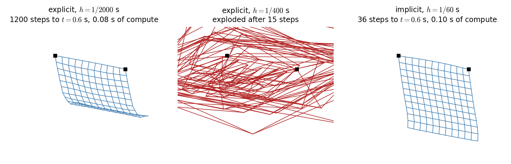
When the Spring Stiffens: Nonlinear Oscillators
cf. linear oscillator: \(u''=-\omega^2u\)
Lossless nonlinear: \(u''=-F(u)\).
Multiply both sides by \(u'\): \[\begin{aligned}
u'u''+F(u)\,u' &= 0 \\
\Leftrightarrow \frac{d}{dt}\Big[\underbrace{\tfrac12(u')^2}_{T}+\underbrace{\int_0^uF(\eta)\,d\eta}_{V}\Big] &= 0,
\end{aligned}\] so the energy \(H=T+V\) is conserved.
Stiffening spring (Duffing): \[ u''=-\omega_0^2u-\omega_1^4u^3, \qquad V=\tfrac{\omega_0^2}{2}u^2+\tfrac{\omega_1^4}{4}u^4 \]
Remark. Nonlinear effects
Larger amplitude \(\Rightarrow\) pitch glide, new partials.
Linear systems only output the input frequency.
Show code
fs, k = 44100, 1 / 44100
w0 = 2 * np.pi * 100
w1 = np.sqrt(w0)                                       # cubic term = linear term at |u| = 1

def duffing(u0, n):
    u = np.zeros(n); u[0] = u[1] = u0
    for i in range(1, n - 1):                          # conservative scheme, explicit update
        q = 1 + 0.5 * w1**4 * k**2 * u[i]**2
        u[i + 1] = (2 - (w0 * k)**2) * u[i] / q - u[i - 1]
    return u

n = 16384
f = np.fft.rfftfreq(n, k)
fig, ax = plt.subplots(figsize=(4.8, 2.3))
for i, (u0, col) in enumerate([(0.01, "k"), (1.0, "steelblue"), (2.5, "darkorange"), (6.0, "firebrick")]):
    u = duffing(u0, n)
    U = np.abs(np.fft.rfft(u * np.hanning(n)))
    ax.plot(f, 20 * np.log10(U / U.max() + 1e-9) - 70 * i, color=col, lw=1, label=f"$u_0={u0:g}$")
ax.set_xlim(0, 2200); ax.set_ylim(-350, 5); ax.set_yticks([])
ax.set_xlabel("frequency (Hz)"); ax.set_title("spectra (offset): pitch rises, partials appear", fontsize=9)
ax.legend(fontsize=7, loc="upper right")
plt.tight_layout()
plt.show()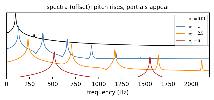
Why Energy-Conserving Schemes Pay Off
Three ways to discretize \(u''=-\omega_1^4u^3\):
| scheme | update | energy |
|---|---|---|
| \(\delta_{tt}u=-\omega_1^4u^3\) | explicit | none known |
| \(\delta_{tt}u=-\omega_1^4u^2\,\mu_{t\cdot}u\) | explicit | conserved, \(\ge0\) |
Second row, solved for \(u^{n+1}\): \[ u^{n+1}=\frac{2u^n}{1+\omega_1^4k^2(u^n)^2/2}-u^{n-1} \] \[ \mathfrak{h}=\tfrac12(\delta_{t-}u)^2+\tfrac{\omega_1^4}{4}(u^n)^2(u^{n-1})^2\ \ge0 \]
The payoff
Unconditionally stable, at no extra cost.
Show code
w1, k, u0 = np.sqrt(20 * np.pi), 1 / 44100, 704.8165
c4 = w1**4 * k**2
N = 900_000                                             # about 20 s at 44.1 kHz

# three algebraically identical ways to write the explicit update, and the conservative one
updates = {"first row, $(2-cu^2)u$": lambda u1, u2: (2 - c4 * u1**2) * u1 - u2,
           "first row, $(2-cuu)u$": lambda u1, u2: (2 - c4 * u1 * u1) * u1 - u2,
           "first row, $2u-cu^3$": lambda u1, u2: 2 * u1 - c4 * u1**3 - u2,
           "second row (conservative)": lambda u1, u2: 2 * u1 / (1 + 0.5 * c4 * u1 * u1) - u2}

def cubic(update):
    u = [u0, u0]
    for n in range(N - 2):
        u.append(update(u[-1], u[-2]))
        if abs(u[-1]) > 1e4:
            break
    return np.array(u)

blk = 4410                                              # 0.1 s blocks
fig, axs = plt.subplots(2, 1, figsize=(4.4, 3.4), height_ratios=[1.3, 1])
for (name, update), col in zip(updates.items(), ["#f1948a", "#e74c3c", "#922b21", "steelblue"]):
    u = cubic(update)
    peaks = [np.abs(u[i:i + blk]).max() for i in range(0, len(u) - 1, blk)]
    blew = len(u) < N
    axs[0].plot(0.1 * np.arange(len(peaks)), peaks, "-", color=col, lw=1.5,
                label=name + (f": blows up at {len(u) * k:.1f} s" if blew else ": bounded"))
    if not blew:
        hn = 0.5 * (np.diff(u) / k)**2 + 0.25 * w1**4 * u[1:]**2 * u[:-1]**2
        axs[1].plot(np.arange(len(hn))[::50] * k, ((hn - hn[0]) / hn[0])[::50], ".", color=col, ms=1)
axs[0].set_ylim(0, 2600); axs[0].set_ylabel("peak $|u|$")
axs[0].set_title("cubic oscillator at 44.1 kHz", fontsize=9)
axs[0].legend(fontsize=6.5, loc="upper left")
axs[1].set_xlabel("time (s)"); axs[1].set_ylabel("rel. energy change")
axs[1].set_title("conservative scheme: rounding only", fontsize=9)
plt.tight_layout()
plt.show()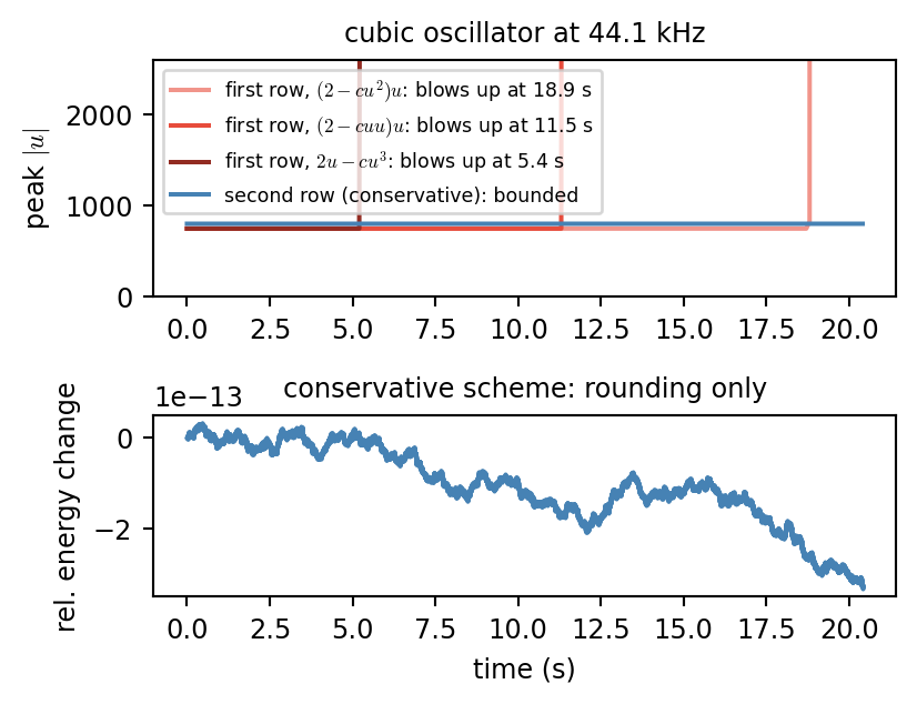
Contact: Hammers and Mallets
Felt stiffens as it is compressed, and pushes only while in contact: \[ F=\omega_H^{\alpha+1}\,\bigl[u_H-u\bigr]_+^{\alpha},\qquad [x]_+=\max(x,0) \] \[ u''=-\omega_0^2u+M_rF,\qquad u_H''=-F \] (\(M_r\): hammer to target mass ratio, \(\alpha\approx2\) to \(4\).)
Remark. Energy
Explicit, and conserves energy up to a tiny jump at contact and release.
Show code
fs, k = 44100, 1 / 44100
w0, MR, wH, a = 2 * np.pi * 400, 0.2, 3000.0, 3.0

def hammer(vH, N=1200, uH0=-1e-4):
    u, uH, Fs = np.zeros(N), np.zeros(N), np.zeros(N)
    uH[0], uH[1] = uH0, uH0 + k * vH
    for n in range(1, N - 1):
        F = wH**(1 + a) * max(uH[n] - u[n], 0.0)**a
        uH[n + 1] = 2 * uH[n] - uH[n - 1] - k**2 * F
        u[n + 1] = (2 - (w0 * k)**2) * u[n] - u[n - 1] + MR * k**2 * F
        Fs[n] = F
    return u, Fs

fig, axs = plt.subplots(2, 1, figsize=(4.4, 3.6))
for vH, col in [(0.25, "lightsteelblue"), (1.0, "steelblue"), (4.0, "navy")]:
    u, Fs = hammer(vH)
    on = np.nonzero(Fs)[0]
    axs[0].plot(1e3 * (np.arange(len(Fs)) - on[0]) * k, Fs / Fs.max(), color=col, lw=1.5,
                label=f"speed {vH:g}: contact {1e3 * (on[-1] - on[0] + 1) * k:.1f} ms")
    spec = np.abs(np.fft.rfft(Fs, 8192))
    axs[1].plot(np.fft.rfftfreq(8192, k) / 1e3, 20 * np.log10(spec / spec[0] + 1e-9), color=col, lw=1.5)
axs[0].set_xlim(-0.2, 3); axs[0].set_xlabel("time from contact (ms)"); axs[0].set_yticks([])
axs[0].set_title("normalized contact force", fontsize=9); axs[0].legend(fontsize=7)
axs[1].set_xlim(0, 8); axs[1].set_ylim(-60, 3); axs[1].set_xlabel("frequency (kHz)"); axs[1].set_ylabel("dB")
axs[1].set_title("force spectrum: harder strike, brighter sound", fontsize=9)
plt.tight_layout()
plt.show()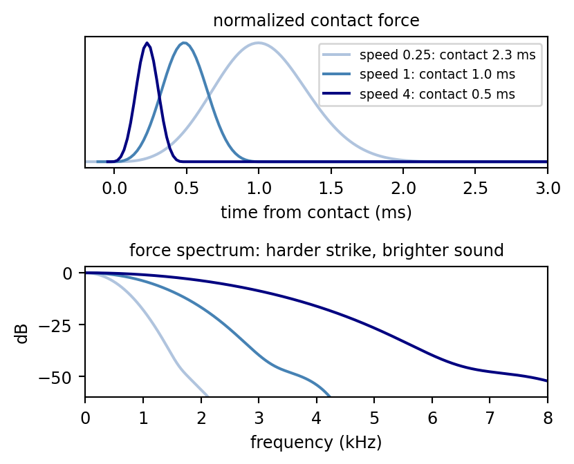
Friction: How a Bow Keeps a String Going
\[ u''=-\omega_0^2u-F_B\,\phi(v_{\mathrm{rel}}),\qquad v_{\mathrm{rel}}=u'-v_B \]
Passive friction: \(\phi(\eta)\,\eta\ge0\). Energy enters only through the bow speed \(v_B\).
Centered scheme \(\ \delta_{tt}u=-\omega_0^2u-F_B\,\phi(\delta_{t\cdot}u-v_B)\) is stable but implicit: each step solves for \(v=v_{\mathrm{rel}}\) \[ g(v)=\tfrac{2}{k}v+F_B\,\phi(v)+b=0 \] (\(b\) from known values). Newton (class 5), warm started:
Unique solution if \(k\le 2/\bigl(F_B\max_\eta(-\phi'(\eta))\bigr)\).
Show code
fs, k = 44100, 1 / 44100
f0, FB, vB, sig = 200.0, 500.0, 0.2, 100.0
A = np.sqrt(2 * sig) * np.exp(0.5)
phi = lambda v: A * v * np.exp(-sig * v**2)                      # soft friction curve, max 1
dphi = lambda v: A * (1 - 2 * sig * v**2) * np.exp(-sig * v**2)

def bowed(FB, N=int(0.1 * fs)):
    u, vr = np.zeros(N), np.zeros(N)
    v = 0.0
    for n in range(1, N - 1):
        b = (2 * np.pi * f0)**2 * u[n] - 2 / k**2 * (u[n] - u[n - 1]) + 2 / k * vB
        for _ in range(20):                                      # Newton on g(v) = 0
            dv = (2 / k * v + FB * phi(v) + b) / (2 / k + FB * dphi(v))
            v -= dv
            if abs(dv) < 1e-12:
                break
        u[n + 1] = 2 * k * (v + vB) + u[n - 1]
        vr[n] = v
    return u, vr

fig = plt.figure(figsize=(4.6, 3.9))
ax0 = fig.add_subplot(3, 2, 1)
eta = np.linspace(-0.6, 0.6, 400)
ax0.plot(eta, phi(eta), color="k")
ax0.set_title("friction $\\phi(v_{\\mathrm{rel}})$", fontsize=8); ax0.set_xticks([0]); ax0.set_yticks([-1, 0, 1])
ax0.axhline(0, color="gray", lw=0.4); ax0.axvline(0, color="gray", lw=0.4)
ax1 = fig.add_subplot(3, 2, 2)
for F_, col in [(200, "lightsteelblue"), (500, "steelblue"), (1000, "navy")]:
    u, _ = bowed(F_)
    ax1.plot(1e3 * np.arange(len(u))[-600:] * k, u[-600:] / np.abs(u[-600:]).max(), color=col, lw=1, label=f"$F_B$={F_}")
ax1.set_title("bow force shapes the wave", fontsize=8); ax1.set_yticks([]); ax1.set_xticks([])
ax1.legend(fontsize=5.5, loc="lower left")
u, vr = bowed(FB)
t = 1e3 * np.arange(len(u)) * k
slip = np.abs(vr) > 0.05
for row, (y, lab) in enumerate([(u * 1e3, "$u$ (mm)"), (vr, "$v_{\\mathrm{rel}}$")]):
    ax = fig.add_subplot(3, 1, row + 2)
    ax.plot(t, y, color="k", lw=1)
    ax.fill_between(t, y.min(), y.max(), where=slip, color="gray", alpha=0.25, lw=0)
    ax.set_ylabel(lab); ax.set_xlim(40, 100)
    if row == 0:
        ax.set_title("stick and slip (shaded: slipping)", fontsize=8); ax.set_xticks([])
    else:
        ax.set_xlabel("time (ms)")
plt.tight_layout()
plt.show()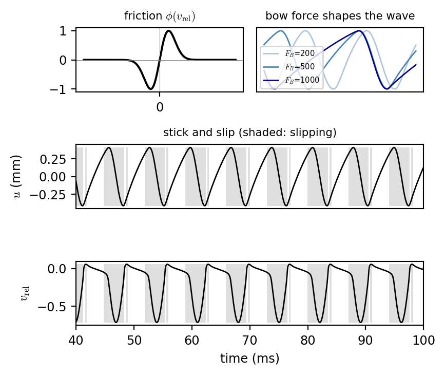
Remark. Auto oscillation
A steady bow speed alone produces a periodic sawtooth-like motion.
How a Sound Starts: Bifurcations
Parameter dependent ODE \(\ \mathbf{y}'=F(\mathbf{y};\mu)\): bow force, blowing pressure, damping.
- Near an equilibrium: \(\mathbf{y}'\approx J(\mu)(\mathbf{y}-\mathbf{y}^*)\), the model equation with \(\lambda=\operatorname{eig}J\).
- Bifurcation: as \(\mu\) moves, an eigenvalue crosses the imaginary axis and the behavior changes qualitatively.
- Hopf: a complex pair crosses; silence becomes a self sustained oscillation, a limit cycle.
Rayleigh’s bowed or blown oscillator (1877): \[ u''=(\mu-u'^2)\,u'-u \] \(\mu u'\) pumps energy in (negative friction), \(-u'^3\) limits it. Amplitude \(\approx\sqrt{4\mu/3}\).
Remark. Numerics moves the threshold
- Forward Euler: onset at \(\mu\approx-h\) (sound from nothing).
- Backward Euler: onset at \(\mu\approx+h\) (needs a harder bow).
- Other bifurcations: saddle node (hysteresis), period doubling toward chaos (multiphonics).
Show code
def rayleigh(u, v, mu):
    return v, (mu - v**2) * v - u

def fe_step(u, v, h, mu):
    du, dv = rayleigh(u, v, mu)
    return u + h * du, v + h * dv

def rk4_step(u, v, h, mu):
    a1, b1 = rayleigh(u, v, mu)
    a2, b2 = rayleigh(u + h / 2 * a1, v + h / 2 * b1, mu)
    a3, b3 = rayleigh(u + h / 2 * a2, v + h / 2 * b2, mu)
    a4, b4 = rayleigh(u + h * a3, v + h * b3, mu)
    return u + h / 6 * (a1 + 2 * a2 + 2 * a3 + a4), v + h / 6 * (b1 + 2 * b2 + 2 * b3 + b4)

def be_step(u, v, h, mu):                      # Newton on the 2x2 implicit system
    U, W = u.copy(), v.copy()
    for _ in range(6):
        g1 = U - u - h * W
        g2 = W - v - h * ((mu - W**2) * W - U)
        d = 1 - h * (mu - 3 * W**2)            # Jacobian [[1, -h], [h, d]]
        det = d + h * h
        U, W = U - (d * g1 + h * g2) / det, W - (g2 - h * g1) / det
    return U, W

def amplitude(step, h, mu, T=300):            # run, then take max |u| over the last 20 s
    u, v = np.full_like(mu, 0.3), np.zeros_like(mu)
    N, amp = int(T / h), np.zeros_like(mu)
    for n in range(N):
        u, v = step(u, v, h, mu)
        if n > N - int(20 / h):
            amp = np.maximum(amp, np.abs(u))
    return amp

fig, ax = plt.subplots(figsize=(4.6, 2.1))
mu = np.linspace(-0.6, 1.0, 161)
ax.plot(mu, amplitude(rk4_step, 0.02, mu), "k", lw=2, label="exact")
ax.plot(mu, amplitude(fe_step, 0.2, mu), color=COL["forward Euler"], lw=1.6, label="forward Euler, $h=0.2$")
ax.plot(mu, amplitude(be_step, 0.2, mu), color=COL["backward Euler"], lw=1.6, label="backward Euler, $h=0.2$")
ax.set_xlabel("$\\mu$ (bow force)"); ax.set_ylabel("amplitude")
ax.set_title("bifurcation diagram", fontsize=9); ax.legend(fontsize=7, loc="upper left")
plt.tight_layout()
plt.show()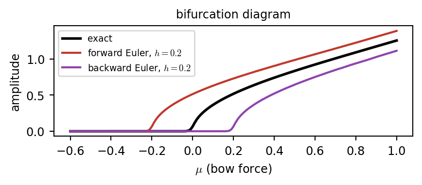
Learning the Right-Hand Side: Neural ODEs
Given an ODE \(\mathbf{x}'=f(\mathbf{x})\)
we want to learn \(f\) from data \((\mathbf{x}_0,\mathbf{x}_1)\), \((\mathbf{x}_1,\mathbf{x}_2)\), \(\dots\)
Recall a forward Euler step: \(\mathbf{x}_{l+1}=\mathbf{x}_l+h\,f(\mathbf{x}_l)\).
ResNet is forward Euler: \(\ \mathbf{x}_{l+1}=\mathbf{x}_l+h\,f_\theta(\mathbf{x}_l)\).
Layers are time steps.
Neural ODE: make the right-hand side a network and use a real solver: \[ \mathbf{y}'=f_\theta(\mathbf{y}),\qquad \mathbf{y}(T)=\texttt{ODESolve}(f_\theta,\mathbf{y}_0,T) \] Train by backpropagating through the solver steps, or by the adjoint ODE solved backward in time (class 11).
Remark. The old rules still apply
\(\operatorname{eig}(\partial f_\theta/\partial\mathbf{y})\) sets stability and stiffness, and long rollouts drift (see the plot on the right.)
Show code
import torch
torch.manual_seed(0); torch.set_default_dtype(torch.float64)
h = 0.1
rng = np.random.default_rng(0)
energy = lambda q, p: 0.5 * p**2 - np.cos(q)

def rk4_t(f, y, h):
    k1 = f(y); k2 = f(y + h / 2 * k1); k3 = f(y + h / 2 * k2); k4 = f(y + h * k3)
    return y + h / 6 * (k1 + 2 * k2 + 2 * k3 + k4)

f_true = lambda y: torch.stack([y[:, 1], -torch.sin(y[:, 0])], 1)
Y0 = torch.tensor(np.c_[rng.uniform(-2.2, 2.2, 400), rng.uniform(-1.6, 1.6, 400)])
Y1 = Y0.clone()
for _ in range(20):                                   # data: exact state 0.1 s later
    Y1 = rk4_t(f_true, Y1, h / 20)

mlp = lambda i, o: torch.nn.Sequential(torch.nn.Linear(i, 64), torch.nn.Tanh(),
                                       torch.nn.Linear(64, 64), torch.nn.Tanh(), torch.nn.Linear(64, o))
f_net, V_net = mlp(2, 2), mlp(1, 1)                   # neural ODE, learned potential

def acc(q):                                            # -dV/dq by autodiff
    q = q if q.requires_grad else q.detach().requires_grad_(True)
    return -torch.autograd.grad(V_net(q[:, None]).sum(), q, create_graph=True)[0]

def leapfrog_t(y, h):
    q, p = y[:, 0], y[:, 1]
    p = p + h / 2 * acc(q); q = q + h * p; p = p + h / 2 * acc(q)
    return torch.stack([q, p], 1)

for net, step in [(f_net, lambda y: rk4_t(f_net, y, h)), (V_net, lambda y: leapfrog_t(y, h))]:
    opt = torch.optim.Adam(net.parameters(), 3e-3)
    for it in range(1500):                             # one step ahead loss
        opt.zero_grad(); loss = ((step(Y0) - Y1)**2).mean(); loss.backward(); opt.step()

ya = yb = torch.tensor([[1.5, 0.0]])
Ea, Eb = [], []
for n in range(3000):                                  # long rollout, about 40 periods
    with torch.no_grad():
        ya = rk4_t(f_net, ya, h)
    yb = leapfrog_t(yb, h).detach()
    Ea.append(energy(*ya[0].numpy())); Eb.append(energy(*yb[0].numpy()))
E0 = energy(1.5, 0.0)
tt = h * np.arange(1, 3001)
fig, ax = plt.subplots(figsize=(4.8, 2.6))
ax.plot(tt, np.array(Ea) - E0, color=COL["RK4"], lw=1.4, label="neural ODE $f_\\theta$ + RK4")
ax.plot(tt, np.array(Eb) - E0, color=COL["leapfrog"], lw=1.4, label="learned $V_\\theta$ + leapfrog")
ax.axhline(0, color="gray", lw=0.5)
ax.set_xlabel("time"); ax.set_ylabel("energy error")
ax.set_title("pendulum, trained on one step pairs, rolled out 3000 steps", fontsize=9)
ax.legend(fontsize=8, loc="upper left")
plt.tight_layout()
plt.show()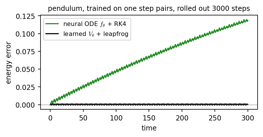
Hamiltonian and Lagrangian NNs
Learn the structure, not just \(F\):
learn a potential \(V_\theta(q)\) and step with leapfrog.
use autodiff to get the force \(-dV/dq\) (cf. class 11).