Partial Differential Equations II

Topics in Digital Heritage:
Numerical Methods for Digital Reconstruction

Jin Woo Lee

KAIST

Fall 2026

Recap

Last Time: The Ideal String

p = np.arange(1, 25)
z = jn_zeros(0, 6).tolist() + jn_zeros(1, 6).tolist() + jn_zeros(2, 6).tolist() + jn_zeros(3, 5).tolist()
rows = [("ideal string", p, COL["string"]),
        ("piano string\n(exaggerated)", p * np.sqrt(1 + 0.01 * p**2) / np.sqrt(1.01), COL["stiff"]),
        ("bar, free ends\n(xylophone)", bar_modes(200)[0][:8] / bar_modes(200)[0][0], COL["bar"]),
        ("circular drum", np.sort(z) / jn_zeros(0, 1)[0], COL["membrane"])]
fig, ax = plt.subplots(figsize=(5.2, 3.2))
for i, (name, f, col) in enumerate(rows):
    y = -i
    for fp in f[f <= 12.5]:
        ax.plot([fp, fp], [y - 0.32, y + 0.32], color=col, lw=2)
    ax.text(-0.3, y, name, ha="right", va="center", fontsize=8.5, color=col)
for m in range(1, 13):
    ax.axvline(m, color="0.85", lw=0.6, ls="--", zorder=0)
ax.set_xlim(0, 12.6); ax.set_ylim(-3.6, 0.6); ax.set_yticks([])
ax.set_xlabel("frequency / fundamental (dashed: harmonics)")
ax.set_title("where the partials are", fontsize=9)
plt.tight_layout()
plt.show()

f = np.linspace(50, 8000, 300)
s0, s1 = loss_params(110, 0, 5.0, 110, 1.0, 4000)
T60 = 3 * np.log(10) / (s0 + s1 * (2 * np.pi * f)**2 / 220**2)
fig, ax = plt.subplots(figsize=(3.8, 3.2))
ax.plot(f / 1e3, np.full_like(f, 3.0), color=COL["string"], lw=2, label="last class: $-2\\sigma_0u_t$")
ax.plot(f / 1e3, T60, color=COL["stiff"], lw=2, label="real string: high partials\ndie first")
ax.set_xlabel("frequency (kHz)"); ax.set_ylabel("$T_{60}$ (s)"); ax.set_ylim(0, 5.5)
ax.set_title("how long each partial rings", fontsize=9); ax.legend(fontsize=7.5)
plt.tight_layout()
plt.show()

Today

Add stiffness (inharmonic partials) and frequency dependent loss (darkening tone), then go briefly to 2D (drums, plates). Same toolbox: difference operators, matrices, boundary conditions, energy, stability.

A Tour of Audio PDEs

system	PDE	instruments	covered
ideal string	\(u_{tt}=\gamma^2u_{xx}\)	guitar, harp (roughly)	class 14
stiff string	\(u_{tt}=\gamma^2u_{xx}-\kappa^2u_{xxxx}\)	piano	today
bar	\(u_{tt}=-\kappa^2u_{xxxx}\)	xylophone, marimba, tuning fork	today
frequency dependent loss	\(\dots-2\sigma_0u_t+2\sigma_1u_{txx}\)	every real instrument	today
helical spring	coupled fourth order system	spring reverb
acoustic tube	\(\frac{1}{S}(S\,p_x)_x=\frac{1}{c^2}p_{tt}\) (Webster)	winds, the vocal tract	class 19
membrane	\(u_{tt}=\gamma^2\nabla^2u\)	drums, timpani	today (2D)
plate	\(u_{tt}=-\kappa^2\nabla^4u\)	gongs, plate reverb	today (2D)
air in a room	\(p_{tt}=c^2\nabla^2p\) (3D)	rooms, halls	class 16

Today’s ILO

• Explain how a fourth order term causes dispersion and inharmonicity, and implement schemes for bars and stiff strings with their boundary and stability conditions.
• Set frequency dependent loss from two decay times and evaluate the tone over time.
• Compute modes of non-uniform structures as an eigenproblem of the semidiscrete system, and use them to tune and strike a marimba bar (modal synthesis).
• Extend grid functions to 2D, simulate membranes and plates, and weigh 2D stability limits and cost.
• Choose a method and recall the stability condition for each audio PDE.

Stiffness: Bars and Stiff Strings

The Ideal Bar: A Fourth Derivative

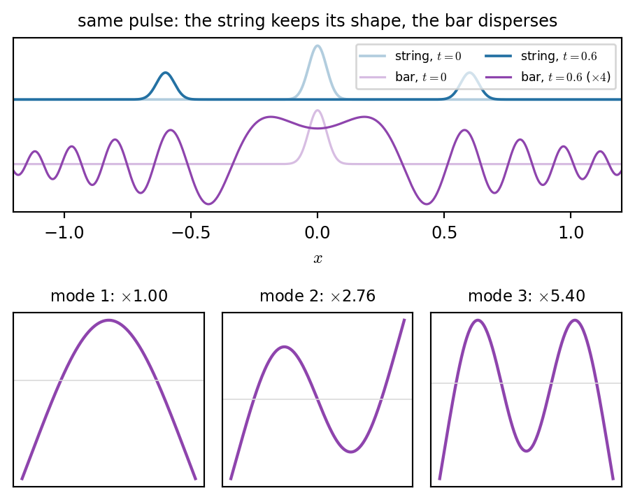
Bending moment \(\propto\) curvature \(u_{xx}\); its second derivative is a force: \[ u_{tt}=-\kappa^2u_{xxxx},\qquad \kappa^2=\frac{EI}{\rho A\,L^4} \] Insert \(e^{j(\omega t+\beta x)}\): \[ \text{string: }\omega=\gamma\beta,\qquad \text{bar: }\omega=\kappa\beta^2 \] Short waves travel faster: physical dispersion (a struck bar chirps; the “boing” of a spring reverb).

Two conditions per end:

end	conditions	example
clamped	\(u=u_x=0\)	tuning fork, kalimba tine
simply supported	\(u=u_{xx}=0\)	(analysis)
free	\(u_{xx}=u_{xxx}=0\)	xylophone bar on cords

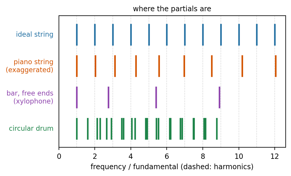
Free/free: \(\ 1:2.76:5.40:8.93\). Clamped/free: \(\ 1:6.27:17.55\).

L, M = 8.0, 4096                                   # a long domain, exact solution by FFT
x = (np.arange(M) - M / 2) * L / M
beta = 2 * np.pi * np.fft.fftfreq(M, L / M)
evolve = lambda u0, omega, t: np.real(np.fft.ifft(np.fft.fft(u0) * np.cos(omega * t)))
u0 = np.exp(-(x / 0.05)**2)
fig = plt.figure(figsize=(4.8, 3.8))
ax = fig.add_subplot(2, 1, 1)
for t, a, mag in [(0, 0.35, 1), (0.6, 1, 4)]:
    ax.plot(x, evolve(u0, beta, t), color=COL["string"], alpha=a, lw=1.4, label=f"string, $t={t}$")
    ax.plot(x, mag * evolve(u0, beta**2 * 0.02, t) - 1.2, color=COL["bar"], alpha=a, lw=1.2,
            label=f"bar, $t={t}$" + (" ($\\times4$)" if mag > 1 else ""))
ax.set_xlim(-1.2, 1.2); ax.set_yticks([]); ax.set_xlabel("$x$")
ax.set_title("same pulse: the string keeps its shape, the bar disperses", fontsize=9)
ax.legend(fontsize=6.5, ncol=2, loc="upper right")
om, V, xb = bar_modes(200)
for i in range(3):
    ax = fig.add_subplot(2, 3, 4 + i)
    ax.plot(xb, V[:, i] / np.abs(V[:, i]).max(), color=COL["bar"], lw=1.6); ax.axhline(0, color="0.85", lw=0.6)
    ax.set_title(f"mode {i + 1}: $\\times${om[i] / om[0]:.2f}", fontsize=8.5); ax.set_xticks([]); ax.set_yticks([])
plt.tight_layout()
plt.show()

Discretizing the Bar

\[ \delta_{tt}u=-\kappa^2\,\delta_{xxxx}u,\qquad \delta_{xxxx}=\delta_{xx}\delta_{xx} \] Explicit, stable for \[ \mu=\frac{\kappa k}{h^2}\le\frac12\quad\Longleftrightarrow\quad h\ge\sqrt{2\kappa k} \]

end	virtual points	matrix
simply supported	\(u_{-1}=-u_1\)	\(\mathbf{D}_{xx}^2\) (Dirichlet)
clamped	\(u_{-1}=u_1\)	first row \([7,-4,1]/h^4\)
free	two, messy	energy form \(\mathbf{K}=\mathbf{D}_2^\top\mathbf{D}_2\)

Energy form: discretize the potential \(\tfrac{\kappa^2}{2}\int u_{xx}^2\) as \(\tfrac{\kappa^2}{2}\sum h(\delta_{xx}u)^2\), then \(\mathbf{M}\mathbf{u}''=-\kappa^2\mathbf{K}\mathbf{u}\). The free conditions come out by themselves (summation by parts in reverse).

# delta_xx at the interior nodes only
D2 = sp.diags([1, -2, 1], [0, 1, 2], shape=(N - 1, N + 1)) / h**2
K = h * D2.T @ D2          # free ends, automatically

f1 = 523.25                                          # C5 xylophone bar
kappa = 2 * np.pi * f1 / 4.7300407**2                # free-free: omega_1 = kappa (4.730)^2
k = 1 / fs
N = int(1 / np.sqrt(2 * kappa * k))                  # largest grid allowed by mu <= 1/2
exact = kappa * np.array([4.7300407, 7.8532046, 10.9956078, 14.1371655, 17.2787597])**2
fig, ax = plt.subplots(figsize=(4.6, 3.4))
for NN, col, ls, lab in [(N, "steelblue", "o-", f"$N={N}$, space only"), (50, "0.6", "s--", "$N=50$ (needs an implicit scheme)")]:
    om = kappa * bar_modes(NN)[0][:5]
    ax.plot(range(1, 6), 1200 * np.log2(om / exact), ls, color=col, ms=4, label=lab)
    if NN == N:
        om_t = 2 / k * np.arcsin(np.minimum(1, k * om / 2))         # time stepping raises each mode
        ax.plot(range(1, 6), 1200 * np.log2(om_t / exact), "o-", color="firebrick", ms=4,
                label=f"$N={N}$, explicit at 44.1 kHz ($\\mu$={kappa * k * N**2:.2f})")
ax.axhline(0, color="k", lw=0.6); ax.axhspan(-100, 100, color="0.94", zorder=0)
ax.set_xticks(range(1, 6)); ax.set_xlabel("mode"); ax.set_ylabel("error (cents)")
ax.set_title(f"C5 bar at 44.1 kHz: explicit allows only $N={N}$", fontsize=9)
ax.legend(fontsize=7, loc="lower left"); ax.set_ylim(-260, 60)
plt.tight_layout()
plt.show()

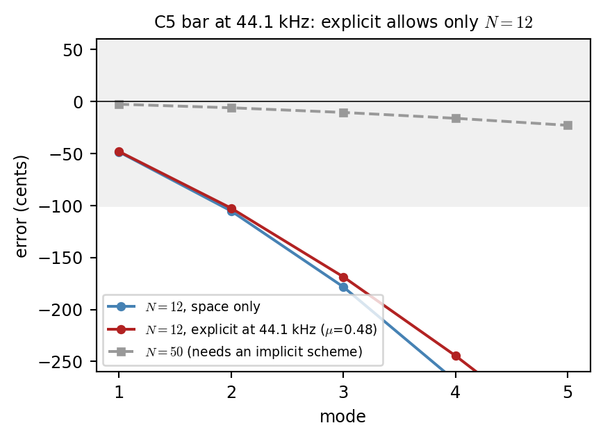
Coarse grid, so high modes come out audibly flat. Remedies: an implicit scheme (free choice of \(h\)) or modal synthesis with accurately computed modes.

Stiff Strings: Why Piano Tuners Stretch Octaves

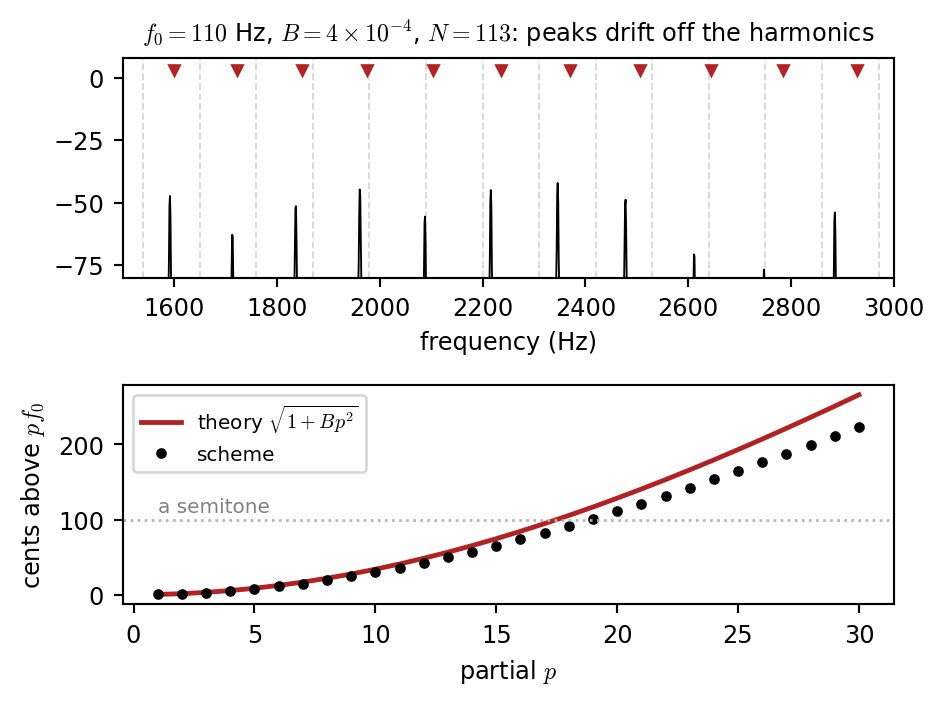
\[ u_{tt}=\gamma^2u_{xx}-\kappa^2u_{xxxx} \] Simply supported ends: \[ f_p=p\,f_0\sqrt{1+Bp^2},\qquad B=\frac{\kappa^2\pi^2}{\gamma^2} \] (piano: \(B\approx10^{-4}\) in the bass to \(10^{-2}\) in the treble).

• Partials are sharp, more so going up: inharmonicity.
• Tuners stretch octaves so that the upper note matches the sharp 2nd partial of the lower one.

Scheme: \(\ \delta_{tt}u=\gamma^2\delta_{xx}u-\kappa^2\delta_{xxxx}u\), stable for \[ h\ge\sqrt{\tfrac12\Bigl(\gamma^2k^2+\sqrt{\gamma^4k^4+16\kappa^2k^2}\Bigr)} \] \(\kappa=0\): \(h\ge\gamma k\) (string). \(\ \gamma=0\): \(h\ge\sqrt{2\kappa k}\) (bar).

f0, B = 110.0, 4e-4
y, N = stiff_string(f0, B, sig0=1.0, dur=1.0, xe=0.13)
fig, axs = plt.subplots(2, 1, figsize=(5.0, 3.8))
Y = np.abs(np.fft.rfft(y * np.hanning(len(y)))); f = np.fft.rfftfreq(len(y), 1 / fs)
p = np.arange(1, 31); f_th = p * f0 * np.sqrt(1 + B * p**2)
for q in p:
    axs[0].axvline(q * f0, color="0.85", ls="--", lw=0.7)
axs[0].plot(f, 20 * np.log10(Y / Y.max() + 1e-9), color="k", lw=0.7)
axs[0].plot(f_th, np.full_like(f_th, 3), "v", color="firebrick", ms=3.5)
axs[0].set_xlim(1500, 3000); axs[0].set_ylim(-80, 8); axs[0].set_xlabel("frequency (Hz)")
axs[0].set_title(f"$f_0=110$ Hz, $B=4\\times10^{{-4}}$, $N={N}$: peaks drift off the harmonics", fontsize=9)
# partials of the scheme from the eigenvalues of the update matrix
gamma, kappa, k, h = 2 * f0, np.sqrt(B) * 2 * f0 / np.pi, 1 / fs, 1 / N
Dxx = sp.diags([1, -2, 1], [-1, 0, 1], shape=(N - 1, N - 1)).toarray() / h**2
lam = np.sort(np.linalg.eigvalsh(gamma**2 * Dxx - kappa**2 * Dxx @ Dxx))[::-1][:30]
f_num = 2 / k * np.arcsin(np.minimum(1, k / 2 * np.sqrt(-lam))) / (2 * np.pi)
axs[1].plot(p, 1200 * np.log2(f_th / (p * f0)), color="firebrick", lw=1.8, label="theory $\\sqrt{1+Bp^2}$")
axs[1].plot(p, 1200 * np.log2(f_num / (p * f0)), "o", color="k", ms=3, label="scheme")
axs[1].axhline(100, color="0.7", ls=":", lw=1); axs[1].text(1, 110, "a semitone", fontsize=7.5, color="0.5")
axs[1].set_xlabel("partial $p$"); axs[1].set_ylabel("cents above $p f_0$")
axs[1].legend(fontsize=7.5, loc="upper left")
plt.tight_layout()
plt.show()

Try It: From String to Bar

Loss and Shape

Frequency Dependent Loss

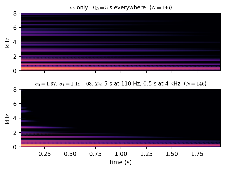
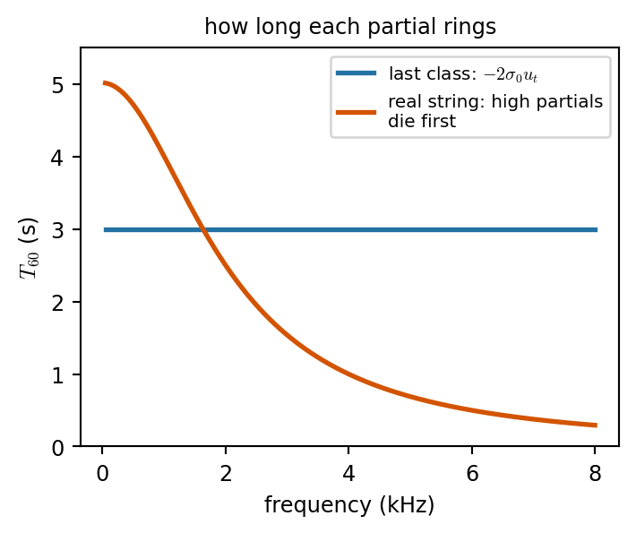
\[ u_{tt}=\gamma^2u_{xx}-\kappa^2u_{xxxx}-2\sigma_0u_t+2\sigma_1u_{txx} \] Decay rate of wavenumber \(\beta\): \(\ \sigma(\beta)\approx\sigma_0+\sigma_1\beta^2\), larger for short waves.

Set from two decay times, e.g. \(T_{60}=5\) s at 110 Hz and \(0.5\) s at 4 kHz: a \(2\times2\) linear system for \((\sigma_0,\sigma_1)\).

Scheme: use \(\delta_{t-}\) in the new term so the update stays explicit: \[ \dots-2\sigma_0\delta_{t\cdot}u+2\sigma_1\delta_{t-}\delta_{xx}u \] Stability: \(h\ge\sqrt{\tfrac12\bigl(a+\sqrt{a^2+16\kappa^2k^2}\bigr)}\) with \(a=\gamma^2k^2+4\sigma_1k\). The energy still only decreases.

f0, B = 110.0, 1e-4
s0, s1 = loss_params(f0, B, 5.0, 110, 0.5, 4000)
runs = [("$\\sigma_0$ only: $T_{60}=5$ s everywhere", 3 * np.log(10) / 5.0, 0.0),
        (f"$\\sigma_0={s0:.2f}$, $\\sigma_1={s1:.1e}$: $T_{{60}}$ 5 s at 110 Hz, 0.5 s at 4 kHz", s0, s1)]
fig, axs = plt.subplots(2, 1, figsize=(5.0, 3.8), sharex=True)
for ax, (title, a0, a1) in zip(axs, runs):
    y, N = stiff_string(f0, B, sig0=a0, sig1=a1, dur=2.0, xe=0.1)
    S, t, f = spectrogram(y)
    ax.pcolormesh(t, f / 1e3, S, vmin=-80, vmax=0, cmap="magma", shading="auto")
    ax.set_ylim(0, 8); ax.set_ylabel("kHz"); ax.set_title(title + f"  ($N={N}$)", fontsize=8.5)
axs[1].set_xlabel("time (s)")
plt.tight_layout()
plt.show()

Tuning a Marimba Bar by Carving It

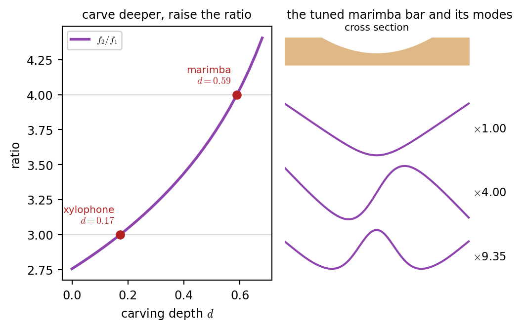
Marimba makers carve an arch under the bar to tune mode 2 to 4× the fundamental (two octaves); xylophones to 3×.

Thickness \(e(x)\): stiffness \(\propto e^3\), mass \(\propto e\): \[ \mathbf{K}=\mathbf{D}_2^\top\operatorname{diag}(h\,e^3)\,\mathbf{D}_2,\qquad \mathbf{M}=\operatorname{diag}(h\,e) \] No closed form, so solve the generalized eigenproblem \[ \mathbf{K}\mathbf{v}=\omega^2\mathbf{M}\mathbf{v} \] (scipy.linalg.eigh(K, M)), and find the depth giving ratio 4 with a root finder (class 5).

• Carving the middle lowers mode 1 most (it bends most there), so the ratio rises.
• Tuning mode 3 too (to 10× on real marimbas) needs more shape parameters: an optimization problem (class 7).

from scipy.optimize import brentq
arch = lambda d: (lambda x: 1 - d * np.clip(1 - ((x - 0.5) / 0.3)**2, 0, None))
ratios = lambda d: (lambda om: om[1:3] / om[0])(bar_modes(150, arch(d))[0])
ds = np.linspace(0, 0.68, 30); R = np.array([ratios(d) for d in ds])
d_mar = brentq(lambda d: ratios(d)[0] - 4, 0.3, 0.7)          # marimba: f2 = 4 f1
d_xyl = brentq(lambda d: ratios(d)[0] - 3, 0.05, 0.4)         # xylophone: f2 = 3 f1
fig, axs = plt.subplots(1, 2, figsize=(5.6, 3.6), width_ratios=[1, 1.1])
axs[0].plot(ds, R[:, 0], color=COL["bar"], lw=2, label="$f_2/f_1$")
for d, r, lab in [(d_xyl, 3, "xylophone"), (d_mar, 4, "marimba")]:
    axs[0].plot(d, r, "o", color="firebrick"); axs[0].axhline(r, color="0.85", lw=0.8, zorder=0)
    axs[0].text(d - 0.02, r + 0.08, f"{lab}\n$d={d:.2f}$", fontsize=7.5, color="firebrick", ha="right")
axs[0].set_xlabel("carving depth $d$"); axs[0].set_ylabel("ratio"); axs[0].legend(fontsize=7, loc="upper left")
axs[0].set_title("carve deeper, raise the ratio", fontsize=9)
om, V, x = bar_modes(150, arch(d_mar))
ax = axs[1]
ax.fill_between(x, 0.6 + 0.25 * arch(d_mar)(x), 0.6, color="burlywood")
ax.text(0.5, 0.92, "cross section", ha="center", fontsize=7.5)
for i in range(3):
    ax.plot(x, 0.25 * V[:, i] / np.abs(V[:, i]).max() - 0.6 * i, color=COL["bar"], lw=1.5)
    ax.text(1.02, -0.6 * i, f"$\\times${om[i] / om[0]:.2f}", fontsize=8.5, va="center")
ax.set_xlim(0, 1.25); ax.axis("off"); ax.set_title("the tuned marimba bar and its modes", fontsize=9)
plt.tight_layout()
plt.show()

Striking the Bar: Mallets and Modal Synthesis

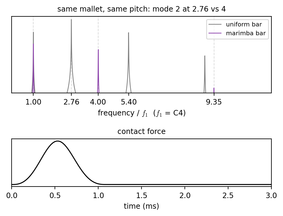
Linear structure + known modes \(\Rightarrow\) modal synthesis, exact pitch with the class 13 recursion: \[ \begin{aligned} q_p^{n+1}=\ &2e^{-\sigma_pk}\cos(\omega_pk)\,q_p^n-e^{-2\sigma_pk}q_p^{n-1}\\ &+k^2\phi_p(x_e)\,F^n \end{aligned} \]

Mallet (class 13): \(\ F=K_H\,[u_H-u(x_e)]_+^{\alpha}\), \(\ u_H''=-F/M_H\).

• A point force enters through a spreading operator \(J_{x_e}\); the bar is read by an interpolation operator \(I_{x_o}\). In modal coordinates: \(\phi_p(x_e)\) and \(\phi_p(x_o)\).
• \(J=I^\top\) keeps the energy balance exact.
• Strike off center: mode 2 is antisymmetric, with a node at the middle.
• Class 18: the same operators couple hammers and bows to a finite difference string.

def strike_bar(profile, f1=261.6, dur=1.2, xe=0.4, xo=0.23, KH=3e10, alpha=2.5, MH=0.02, vH=1.0):
    om, V, x = bar_modes(150, profile)
    keep = om * f1 / om[0] < 2 * np.pi * 18000                # modes below 18 kHz
    om, V = om[keep] * 2 * np.pi * f1 / om[0], V[:, keep]
    sig = 0.6 + 2e-8 * om**2                                  # higher modes decay faster
    phe, pho = V[int(xe * 150)], V[int(xo * 150)]             # spreading / interpolation weights
    k = 1 / fs; c1, c2 = 2 * np.exp(-sig * k) * np.cos(om * k), np.exp(-2 * sig * k)
    q, qp = np.zeros(len(om)), np.zeros(len(om))
    uH, uHp, out, F_hist = -1e-5, -1e-5 - k * vH, np.zeros(int(dur * fs)), []   # just short of contact, moving in
    for n in range(len(out)):
        F = KH * max(uH - phe @ q, 0.0)**alpha                 # contact force
        q, qp = c1 * q - c2 * qp + k**2 * phe * F, q
        uH, uHp = 2 * uH - uHp - k**2 * F / MH, uH
        out[n] = pho @ q; F_hist.append(F)
    return out, np.array(F_hist), om / (2 * np.pi)

uniform = lambda x: np.ones_like(x)
fig, axs = plt.subplots(2, 1, figsize=(4.9, 3.8), height_ratios=[1.6, 1])
for prof, col, lab, off in [(uniform, "0.5", "uniform bar", 0), (arch(d_mar), COL["bar"], "marimba bar", -40)]:
    y, F, fm = strike_bar(prof)                               # struck slightly off center
    Y = np.abs(np.fft.rfft(y * np.hanning(len(y)))); f = np.fft.rfftfreq(len(y), 1 / fs)
    axs[0].plot(f / 261.6, 20 * np.log10(Y / Y.max() + 1e-9) + off, color=col, lw=0.9, label=lab)
    if prof is uniform:
        axs[1].plot(1e3 * np.arange(len(F)) / fs, F / F.max(), color="k", lw=1.2)
for r in [1, 2.76, 4, 9.35]:
    axs[0].axvline(r, color="0.85", ls="--", lw=0.8, zorder=0)
axs[0].set_xlim(0, 12); axs[0].set_ylim(-120, 5); axs[0].set_yticks([])
axs[0].set_xticks([1, 2.76, 4, 5.4, 9.35]); axs[0].set_xlabel("frequency / $f_1$  ($f_1$ = C4)")
axs[0].set_title("same mallet, same pitch: mode 2 at 2.76 vs 4", fontsize=9); axs[0].legend(fontsize=7.5)
axs[1].set_xlim(0, 3); axs[1].set_xlabel("time (ms)"); axs[1].set_yticks([])
axs[1].set_title("contact force", fontsize=9)
plt.tight_layout()
plt.show()

Going 2D: Drums and Plates

Grids in 2D

Grid function \(u_{l,m}^n\approx u(lh,\,mh,\,nk)\).

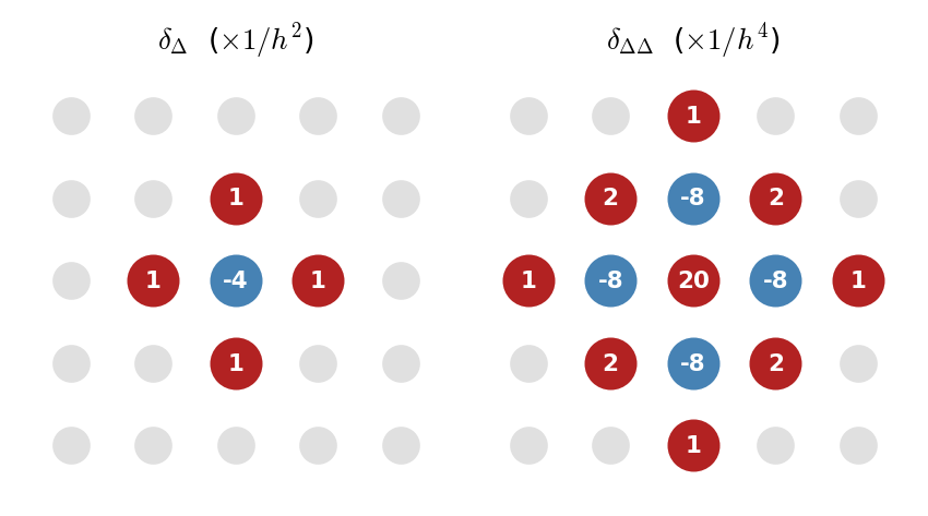
• Laplacian: \(\ \delta_\Delta=\delta_{xx}+\delta_{yy}\) (5 points), the operator of last class’s scan fill.
• Biharmonic: \(\ \delta_{\Delta\Delta}=\delta_\Delta\delta_\Delta\) (13 points), for plates.
• Matrices are Kronecker sums:

D, I = D_xx(n, h), sp.identity(n)
Lap = sp.kron(I, D) + sp.kron(D, I)   # 5 point
Bih = Lap @ Lap                       # 13 point

• Round domains: polar grids or staircase boundaries. Off-grid pickups and forces: bilinear interpolation (class 8).

Cost

Unknowns grow like \((f_s/\gamma)^d\): hundreds in 1D, tens of thousands for a drum in 2D, billions for a room in 3D (class 16).

The 2D Wave Equation: Drums

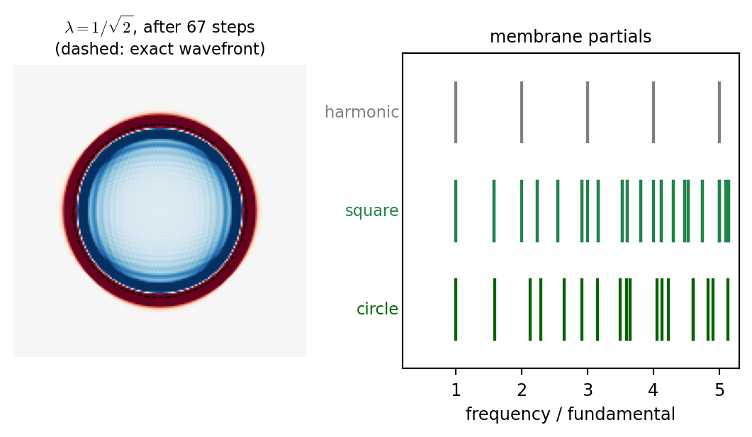
\[ u_{tt}=\gamma^2\nabla^2u\quad\Rightarrow\quad\delta_{tt}u=\gamma^2\delta_\Delta u \] Stable for \[ \lambda=\frac{\gamma k}{h}\le\frac{1}{\sqrt2} \] (the checkerboard mode has twice the 1D eigenvalue).

• Numerical dispersion now depends on direction: exact along the diagonals at \(\lambda=1/\sqrt2\), slow along the axes. No \(\lambda\) is exact everywhere.
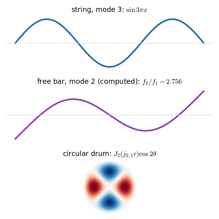
• Modes: square \(\propto\sqrt{p^2+q^2}\); circle \(\propto\) Bessel zeros \(j_{m,n}\). Not harmonic, so drums have a vague pitch (timpani shift them close to harmonic).

n = 161; h = 1 / (n - 1); lam = 1 / np.sqrt(2)
X, Y = np.meshgrid(np.linspace(-0.5, 0.5, n), np.linspace(-0.5, 0.5, n))
u = 0.5 * (1 + np.cos(np.pi * np.clip(np.hypot(X, Y) / 0.04, 0, 1)))    # struck: a smooth bump
up = u.copy(); steps = int(0.3 / (lam * h))
for _ in range(steps):
    un = np.zeros_like(u)
    un[1:-1, 1:-1] = (2 * u[1:-1, 1:-1] - up[1:-1, 1:-1] + lam**2 * (u[2:, 1:-1] + u[:-2, 1:-1]
                      + u[1:-1, 2:] + u[1:-1, :-2] - 4 * u[1:-1, 1:-1]))
    up, u = u, un
fig, axs = plt.subplots(1, 2, figsize=(5.6, 3.2), width_ratios=[1, 1.15])
axs[0].imshow(u, cmap="RdBu_r", vmin=-0.02, vmax=0.02, extent=[-0.5, 0.5, -0.5, 0.5], origin="lower")
s = np.linspace(0, 2 * np.pi, 200); r = steps * lam * h
axs[0].plot(r * np.cos(s), r * np.sin(s), color="k", lw=0.7, ls="--")
axs[0].set_title(f"$\\lambda=1/\\sqrt{{2}}$, after {steps} steps\n(dashed: exact wavefront)", fontsize=8.5); axs[0].axis("off")
pq = np.sort([np.hypot(p_, q_) for p_ in range(1, 9) for q_ in range(1, 9)]) / np.sqrt(2)
circ = np.sort(np.concatenate([jn_zeros(m, 8) for m in range(0, 8)])) / jn_zeros(0, 1)[0]
for i, (name, fr, col) in enumerate([("harmonic", np.arange(1, 7), "0.5"), ("square", pq, COL["membrane"]),
                                     ("circle", circ, "darkgreen")]):
    for v in fr[fr <= 5.2]:
        axs[1].plot([v, v], [-i - 0.3, -i + 0.3], color=col, lw=1.6)
    axs[1].text(0.15, -i, name, ha="right", va="center", fontsize=8.5, color=col)
axs[1].set_xlim(0.2, 5.3); axs[1].set_ylim(-2.6, 0.6); axs[1].set_yticks([])
axs[1].set_xlabel("frequency / fundamental"); axs[1].set_title("membrane partials", fontsize=9)
plt.tight_layout()
plt.show()

Plates: Gongs and Plate Reverb

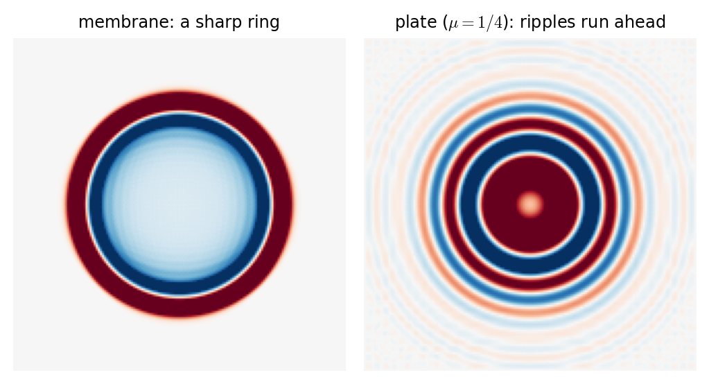
\[ u_{tt}=-\kappa^2\nabla^4u-2\sigma_0u_t+2\sigma_1\nabla^2u_t+J_{x_e}F \] Scheme: \(\ \delta_{tt}u=-\kappa^2\delta_{\Delta\Delta}u+\dots\), stable for \[ \mu=\frac{\kappa k}{h^2}\le\frac14 \]

• Dispersive like the bar: short waves run ahead.
• Plate reverb (EMT 140, 1957): a suspended steel sheet, driven at one point by the audio signal \(F(t)\) and read at two pickups for stereo. The digital version is this scheme.
• Gongs and cymbals at large amplitude become nonlinear (pitch glides, shimmer), the 2D cousin of the Duffing oscillator of class 13.

def lap(v):                                          # 5 point Laplacian times h^2, zero outside
    out = np.zeros_like(v)
    out[1:-1, 1:-1] = v[2:, 1:-1] + v[:-2, 1:-1] + v[1:-1, 2:] + v[1:-1, :-2] - 4 * v[1:-1, 1:-1]
    return out
n = 161; h = 1 / (n - 1)
X, Y = np.meshgrid(np.linspace(-0.5, 0.5, n), np.linspace(-0.5, 0.5, n))
u0 = 0.5 * (1 + np.cos(np.pi * np.clip(np.hypot(X, Y) / 0.06, 0, 1)))
mu = 0.25; u, up = u0.copy(), u0.copy()              # plate, kappa = 1: k = mu h^2
for _ in range(200):
    u, up = 2 * u - up - mu**2 * lap(lap(u)), u
lam = 1 / np.sqrt(2); w, wp = u0.copy(), u0.copy()  # membrane with the same spread
for _ in range(int(0.3 / (lam * h))):
    w, wp = 2 * w - wp + lam**2 * lap(w), w
fig, axs = plt.subplots(1, 2, figsize=(5.4, 3.0))
for ax, field, title in [(axs[0], w, "membrane: a sharp ring"), (axs[1], u, f"plate ($\\mu=1/4$): ripples run ahead")]:
    v = np.abs(field).max() * 0.4
    ax.imshow(field, cmap="RdBu_r", vmin=-v, vmax=v); ax.axis("off"); ax.set_title(title, fontsize=9)
plt.tight_layout()
plt.show()

Try It: Drum and Plate

Choosing a Method

Audio PDEs at a Glance

system	scheme	stable when	grid at 44.1 kHz (example)
string	\(\delta_{tt}u=\gamma^2\delta_{xx}u\)	\(\lambda=\gamma k/h\le1\)	\(\approx100\) points (220 Hz)
stiff string	\(+\,-\kappa^2\delta_{xxxx}u\)	\(h\ge\sqrt{\frac12(\gamma^2k^2+\sqrt{\gamma^4k^4+16\kappa^2k^2})}\)	\(\approx100\) points (110 Hz, \(B=4\times10^{-4}\))
bar	\(\delta_{tt}u=-\kappa^2\delta_{xxxx}u\)	\(\mu=\kappa k/h^2\le\frac12\)	\(\approx12\) points (C5 bar)
membrane	\(\delta_{tt}u=\gamma^2\delta_\Delta u\)	\(\lambda\le\frac{1}{\sqrt2}\)	\(10^4\) to \(10^5\) points
plate	\(\delta_{tt}u=-\kappa^2\delta_{\Delta\Delta}u\)	\(\mu\le\frac14\)	\(10^4\) to \(10^5\) points

All are \(k\le2/\sqrt{\lambda_{\max}}\) for the spatial operator (class 13), and all follow from the energy method too.

Checklist

1. Linear, modes computable (even for a carved bar): modal synthesis, exact pitch.
2. Ideal 1D string or tube: digital waveguide, \(O(1)\) per sample.

3. Nonlinear, coupled, or 2D/3D: finite differences (or finite elements for complex shapes).
4. Always: monitor the discrete energy; keep \(\lambda\) or \(\mu\) near the limit.

Looking Ahead

Where These Ideas Come Back

• Project proposals (next week): any PDE of today can model a heritage instrument or space.
• Wave Propagation: waves spreading in 2D and 3D, reflection, absorbing boundaries, room acoustics.
• 1D Wave Equation and Stability Analysis: derive every condition of the table with von Neumann analysis; numerical dispersion in detail.
• Stringed Instruments: stiff, lossy strings driven by the hammer and bow of class 13 through spreading operators; strings coupled to a soundboard (a plate).
• Wind Instruments: tubes of varying cross section (Webster’s equation, handled like today’s carved bar) driven by a reed.

Recap

Recap on Today’s ILO

• Stiffness: \(u_{xxxx}\) causes dispersion and inharmonicity; bars need only a few grid points (\(\mu\le\tfrac12\)); free ends come for free from the energy form.
• Frequency dependent loss: \(2\sigma_1u_{txx}\) darkens the tone; set \((\sigma_0,\sigma_1)\) from two \(T_{60}\)’s; \(\delta_{t-}\) keeps it explicit.
• Modes of any shape: the eigenproblem \(\mathbf{K}\mathbf{v}=\omega^2\mathbf{M}\mathbf{v}\) tunes a carved marimba bar; modal synthesis plus a mallet plays it.
• 2D: membranes (\(\lambda\le1/\sqrt2\)) and plates (\(\mu\le\tfrac14\)); unknowns grow like \((f_s/\gamma)^2\).
• Choose: modal for linear, waveguides for ideal 1D, finite differences for the rest; always watch the energy.
• Next week: project proposals.