String Instruments and FEM


Topics in Digital Heritage:
Numerical Methods for Digital Reconstruction

Jin Woo Lee

KAIST

Fall 2026

Recap

Last Time: A String in a Vacuum

Stiff, lossy string (class 15): \[ u_{tt}=\gamma^2u_{xx}-\kappa^2u_{xxxx}-2\sigma_0u_t+2\sigma_1u_{txx} \] partials \(f_p=pf_0\sqrt{1+Bp^2}\), explicit if \(h\ge h_{\min}(\gamma,\kappa,\sigma_1,k)\).

Energy form (class 15): discretize the energy, get \(\mathbf{M}\mathbf{u}''=-\mathbf{K}\mathbf{u}\); free ends come out by themselves.

Modes of any shape (class 15): \(\ \mathbf{K}\mathbf{v}=\omega^2\mathbf{M}\mathbf{v}\).

Point forces (class 15): spread with \(J_{x_e}\), read with \(I_{x_o}\).

Lumped exciters (class 13): hammer contact and bow friction on a single oscillator.

Show code
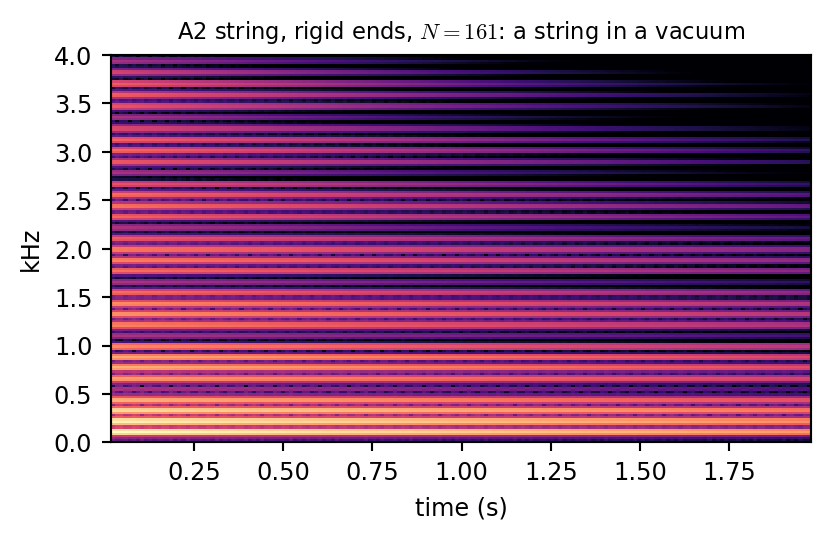
s = guitar_string(1)                                  # A2, rigid at both ends
pluck_ic(s, s.L - 0.13)
y_vac = simulate([s], dur=2.0)["bridge"]
save_wav("recap_rigid", y_vac)
fig, ax = plt.subplots(figsize=(4.4, 2.9))
show_spec(ax, y_vac, f"A2 string, rigid ends, $N={s.N}$: a string in a vacuum")
ax.set_xlabel("time (s)"); ax.set_ylabel("kHz")
plt.tight_layout()
plt.show()

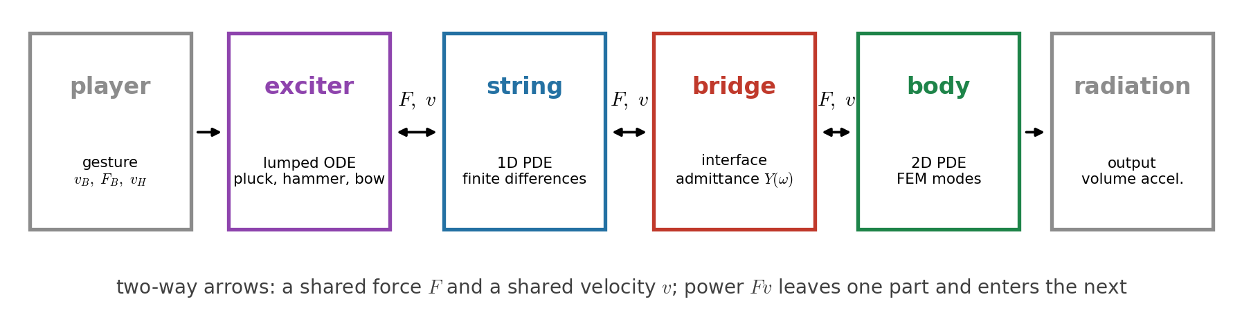
Component Model of a Stringed Instrument

part guitar violin piano model today
exciter finger, pick bow (friction) felt hammer (contact) ODE, one scalar equation per step
string steel or nylon gut, steel 1 to 3 steel strings per note stiff lossy FD string (class 15)
bridge glued to the top stands on the top glued to the soundboard point admittance \(Y(\omega)\)
body top plate + air cavity plates + air soundboard FEM modes, modal bank

Today’s ILO

  • Explain a string instrument as lumped exciters coupled to a distributed string, and couple a pluck, hammer, or bow to a finite difference string through spreading and interpolation operators, solving the contact or friction equation at every step (Newton for the bow).
  • Model a non-rigid bridge by its admittance \(Y(\omega)\), implement it as a bank of modal oscillators sharing a force with the string, and predict and verify how it damps and detunes each partial (including piano unisons).
  • Derive finite elements with linear elements in 1D and 2D, compare consistent and lumped mass with finite differences, and compute the modes of an irregular body from \(\mathbf{K}\boldsymbol{\phi}=\omega^2\mathbf{M}\boldsymbol{\phi}\).
  • Assemble a full string, exciter, bridge, body instrument, justify its stability with an energy argument, and weigh precomputation against per-sample cost.
  • Recognize where the linear model ends: tension modulation and pitch glides.

Exciting the String

Lumped Forces Meet a Distributed String

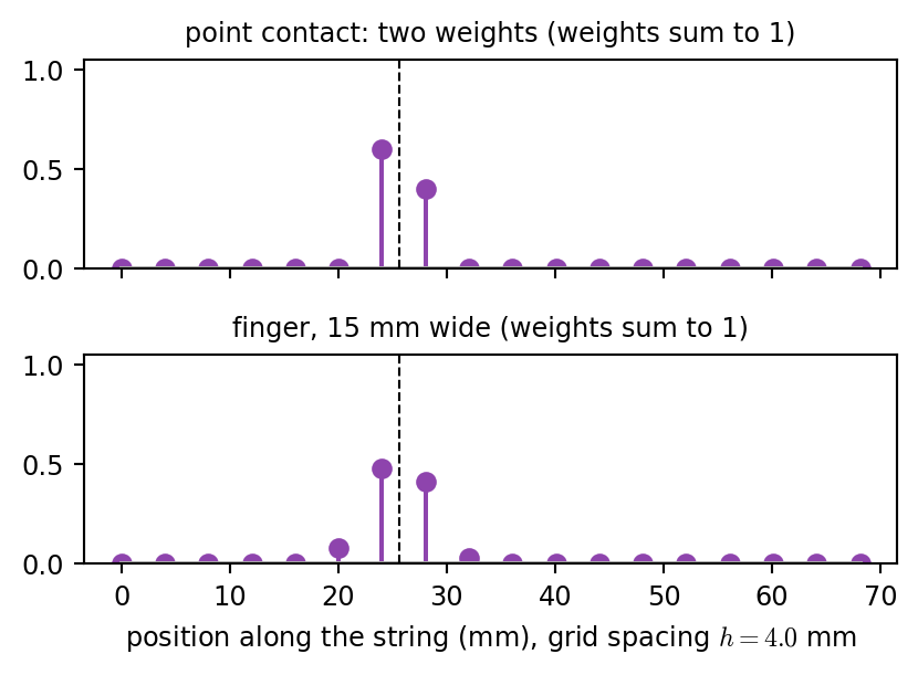
Semi-discrete string with a point force: \[ \mathbf{M}\mathbf{u}''=-\mathbf{K}\mathbf{u}-\mathbf{C}\mathbf{u}'+J\,F \] The exciter only sees the contact value \(I\mathbf{u}\). Choose \(I=J^\top\) (same weights): the power given by the exciter, \(F\,(I\mathbf{u}')\), equals the power received by the string, \((JF)\cdot\mathbf{u}'\).

Each time step

  1. \(\bar{\mathbf{u}}\): string update without \(F\) (explicit, class 15).
  2. One scalar equation for \(F\) at the contact, using \(I\bar{\mathbf{u}}\) (closed form, or Newton).
  3. \(\mathbf{u}^{n+1}=\bar{\mathbf{u}}+\dfrac{k^2}{1+\sigma_0k}\mathbf{M}^{-1}J\,F\).
ub = s.free()                         # 1. explicit string step
F = contact_force(s.J @ ub, ...)      # 2. scalar equation at the contact
ub += s.gain * s.J * F                # 3. spread back (M is diagonal)
Show code
s = guitar_string(1)
xs = s.x[100:118] - s.x[100]; xe = s.x[106] + 0.4 * s.h
J_pt = s.spread(xe)[100:118]                          # point: linear interpolation weights
J_w = s.spread(xe, width=0.015)[100:118]              # a 15 mm wide finger: raised cosine
fig, axs = plt.subplots(2, 1, figsize=(4.4, 3.3), sharex=True)
for ax, J, title in [(axs[0], J_pt, "point contact: two weights"), (axs[1], J_w, "finger, 15 mm wide")]:
    ax.stem(1e3 * xs, J, linefmt=COL["exciter"], markerfmt="o", basefmt="0.7")
    ax.axvline(1e3 * (xe - s.x[100]), color="k", ls="--", lw=0.8)
    ax.set_title(title + f" (weights sum to {J.sum():.0f})", fontsize=9); ax.set_ylim(0, 1.05)
axs[1].set_xlabel("position along the string (mm), grid spacing "
                  f"$h={1e3 * s.h:.1f}$ mm")
plt.tight_layout()
plt.show()

Rule of thumb

Explicit for the distributed part, (semi-)implicit for the lumped part: the implicit solve is one scalar.

Plucking

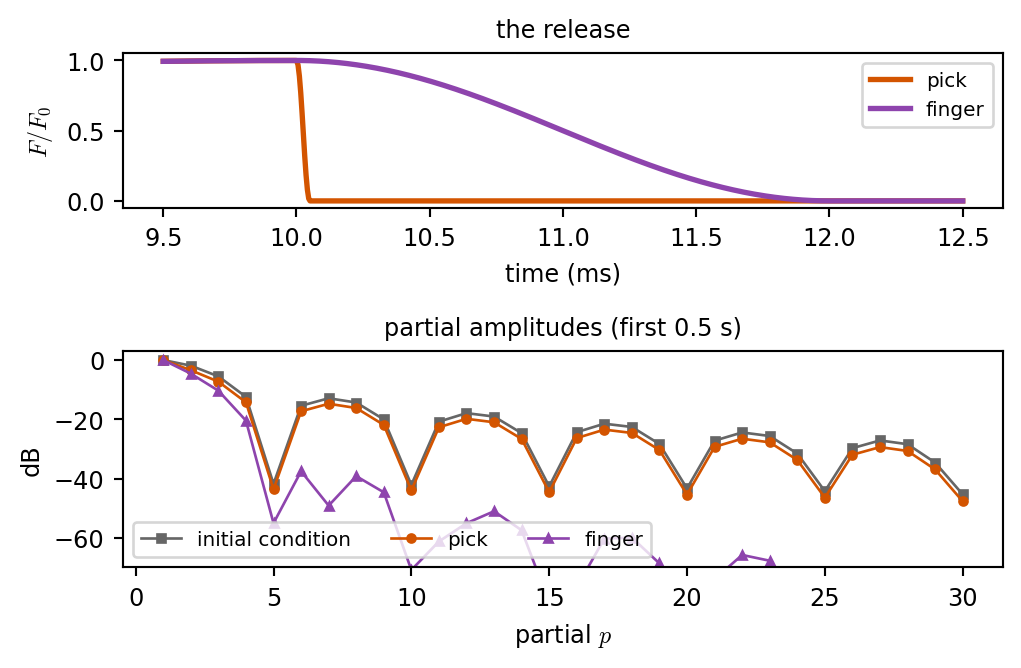
Initial condition: a triangle released at \(t=0\). Instantaneous and perfectly sharp: partial \(p\) gets \(\propto\frac{\sin(p\pi x_e/L)}{p^2}\).

Force: a finger pushes, then the string slides off: \[ F(t)=\begin{cases}\tfrac{F_0}{2}\bigl(1-\cos\tfrac{\pi t}{t_{\text{push}}}\bigr)&\text{push}\\[2pt]\tfrac{F_0}{2}\bigl(1+\cos\tfrac{\pi(t-t_{\text{push}})}{t_{\text{rel}}}\bigr)&\text{release}\end{cases} \] spread over the contact width \(w\).

  • Release time \(t_{\text{rel}}\) low passes in time.
  • Width \(w\) low passes in space.
  • Pick: short and narrow (bright). Flesh: long and wide (dark).
Show code
runs = {}
for name, kind, width, t_rel in [("initial condition", "ic", 0, 0), ("pick", "force", 0.0, 5e-5), ("finger", "force", 0.015, 2e-3)]:
    s = guitar_string(1)
    ex = Pluck(s, s.L - 0.13, F0=1.0, width=width, t_rel=t_rel) if kind == "force" else None
    if kind == "ic":
        pluck_ic(s, s.L - 0.13)
    runs[name] = (simulate([s], dur=2.0, exciters=[ex])["bridge"], ex)
    save_wav("pluck_" + name.split()[0], runs[name][0])
fig, axs = plt.subplots(2, 1, figsize=(5.4, 3.6), height_ratios=[1, 1.4])
t = np.linspace(0.0095, 0.0125, 600)
for (name, (y, ex)), col in zip(list(runs.items())[1:], [COL["stiff"], COL["exciter"]]):
    axs[0].plot(1e3 * t, [ex.force(ti) for ti in t], color=col, lw=2, label=name)
axs[0].set_xlabel("time (ms)"); axs[0].set_ylabel("$F/F_0$"); axs[0].legend(fontsize=7.5)
axs[0].set_title("the release", fontsize=9)
for (name, (y, ex)), col, mk in zip(runs.items(), ["0.4", COL["stiff"], COL["exciter"]], ["s", "o", "^"]):
    axs[1].plot(np.arange(1, 31), partial_amps(y, 110.0, B=5e-5), mk + "-", color=col, ms=3, lw=1, label=name)
axs[1].set_xlabel("partial $p$"); axs[1].set_ylabel("dB"); axs[1].set_ylim(-70, 3)
axs[1].legend(fontsize=7.5, ncol=3, loc="lower left"); axs[1].set_title("partial amplitudes (first 0.5 s)", fontsize=9)
plt.tight_layout()
plt.show()
initial condition

pick (\(t_{\text{rel}}=0.05\) ms, point)

finger (\(t_{\text{rel}}=2\) ms, \(w=15\) mm)

Hammer

Class 13 contact, now on a string: \[ F=K_H\bigl[u_H-I\mathbf{u}\bigr]_+^{\alpha},\qquad M_Hu_H''=-F \] and \(+JF\) on the string. Explicit:

F = KH * max(uH - J @ s.u, 0.0)**alpha
ub += s.gain * J * F
uH, uHp = 2*uH - uHp - k**2 * F / MH, uH

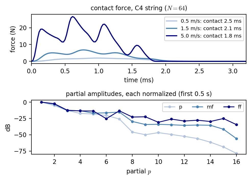
C4 piano string and hammer (measured): \(M_H=2.97\) g, \(K_H=4.5\times10^9\), \(\alpha=2.5\), struck at \(0.12L\).

  • Harder strike: shorter contact, brighter tone.
  • Several peaks: waves reflected from the near end come back and push the hammer.
Show code
fig, axs = plt.subplots(2, 1, figsize=(5.2, 3.8), height_ratios=[1, 1.1])
for i, (vH, col, tag) in enumerate([(0.5, "lightsteelblue", "p"), (1.5, "steelblue", "mf"), (5.0, "navy", "ff")]):
    s = String(f0=261.6, L=0.62, rhoA=6.3e-3, B=4e-4, T60=(12.0, 1.5))
    ham = Hammer(s, 0.12 * s.L, vH=vH)
    y = simulate([s], dur=2.0, exciters=[ham])["bridge"]
    save_wav(f"hammer_{tag}", y)
    F = np.array(ham.F); on = np.nonzero(F)[0]
    axs[0].plot(1e3 * np.arange(len(F)) * k, F, color=col, lw=1.6,
                label=f"{vH} m/s: contact {1e3 * (on[-1] - on[0] + 1) * k:.1f} ms")
    axs[1].plot(np.arange(1, 17), partial_amps(y, 261.6, P=16, B=4e-4), "o-", color=col, ms=3, lw=1.2, label=tag)
axs[0].set_xlim(0, 3.2); axs[0].set_xlabel("time (ms)"); axs[0].set_ylabel("force (N)")
axs[0].legend(fontsize=7.5); axs[0].set_title(f"contact force, C4 string ($N={s.N}$)", fontsize=9)
axs[1].set_ylim(-80, 3); axs[1].set_ylabel("dB"); axs[1].legend(fontsize=7.5, ncol=3)
axs[1].set_xlabel("partial $p$"); axs[1].set_title("partial amplitudes, each normalized (first 0.5 s)", fontsize=9)
plt.tight_layout()
plt.show()
p, 0.5 m/s

mf, 1.5 m/s

ff, 5 m/s (each clip normalized)

Bowing

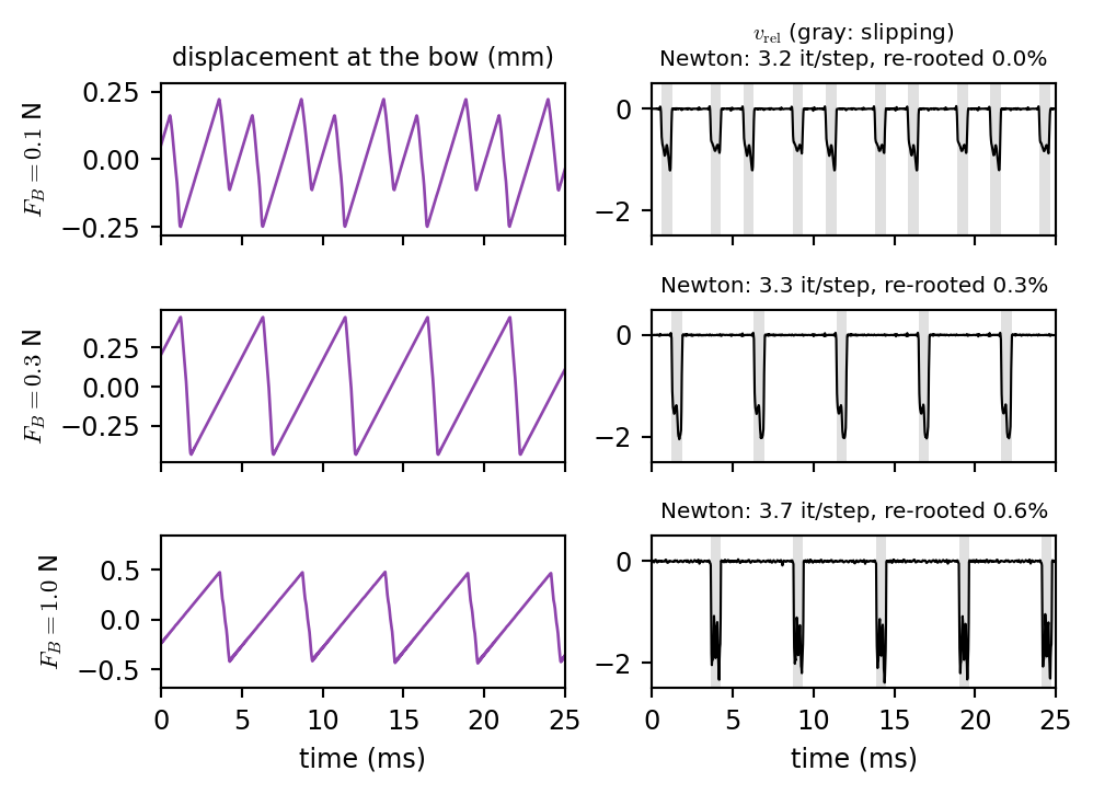
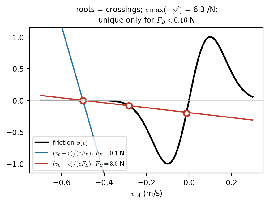
Friction opposes the relative velocity (class 13): \[ -J\,F_B\,\phi(v_{\text{rel}}),\qquad v_{\text{rel}}=I\,\delta_{t\cdot}\mathbf{u}-v_B \] \(\delta_{t\cdot}\) uses \(\mathbf{u}^{n+1}\): implicit, but at one point. Read \(\bar{\mathbf{u}}\) at the bow, \(v_0=\frac{I\bar{\mathbf{u}}-I\mathbf{u}^{n-1}}{2k}-v_B\), then \[ g(v)=v-v_0+c\,F_B\,\phi(v)=0 \] with \(c=\sum_j\frac{J_j^2\,k}{2(1+\sigma_0k)m_j}\) (weights and node masses at the bow). Newton (class 5), warm started from the last step:

for _ in range(20):
    dv = (v - v0 + cF * phi(v)) / (1 + cF * dphi(v))
    v -= dv
    if abs(dv) < 1e-10: break
ub -= s.gain * J * FB * phi(v)

Unique iff \(\ c\,F_B\max(-\phi')<1\). Otherwise keep the root nearest the last one (hysteresis). Spreading over the hair width lowers \(c\).

Show code
s = String(f0=196.0, L=0.325, rhoA=2.7e-3, B=1e-5, T60=(5.0, 1.0))   # violin G string
bow = Bow(s, s.L * 0.88, width=0.008)
c = bow.c
v = np.linspace(-0.7, 0.3, 1000)
fig, ax = plt.subplots(figsize=(4.6, 3.6))
ax.plot(v, phi_b(v), color="k", lw=2, label="friction $\\phi(v)$")
for FB, v0, col in [(0.1, -0.5, COL["string"]), (3.0, -0.5, COL["bridge"])]:
    line = (v0 - v) / (c * FB)
    ax.plot(v, line, color=col, lw=1.5, label=f"$(v_0-v)/(cF_B)$, $F_B={FB}$ N")
    g = v - v0 + c * FB * phi_b(v); r = v[:-1][np.sign(g[:-1]) != np.sign(g[1:])]
    ax.plot(r, phi_b(r), "o", color=col, ms=7, mfc="white", mew=2)
ax.axhline(0, color="0.8", lw=0.6); ax.axvline(0, color="0.8", lw=0.6)
ax.set_ylim(-1.15, 1.15); ax.set_xlabel("$v_{\\mathrm{rel}}$ (m/s)")
ax.set_title(f"roots = crossings; $c\\,\\max(-\\phi')$ = {c * -dphi_b(np.sqrt(1.5 / A_BOW)):.1f} /N:\n"
             f"unique only for $F_B<{1 / (c * -dphi_b(np.sqrt(1.5 / A_BOW))):.2f}$ N", fontsize=9)
ax.legend(fontsize=7.5, loc="lower left")
plt.tight_layout()
plt.show()

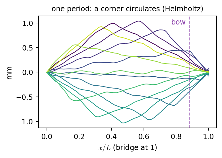
Helmholtz Motion and Stick-Slip

Show code
fig, axs = plt.subplots(3, 2, figsize=(5.2, 3.9), sharex=True)
for row, (FB, (y, bow, s)) in enumerate(bowed.items()):
    t = 1e3 * (np.arange(len(bow.vr)) * k - 1.0)
    axs[row, 0].plot(t, 1e3 * np.array(bow.ub), color=COL["exciter"], lw=1)
    axs[row, 1].plot(t, bow.vr, color="k", lw=0.8)
    axs[row, 1].fill_between(t, -2.5, 0.5, where=np.array(bow.vr) < -0.05, color="0.6", alpha=0.3, lw=0)
    axs[row, 0].set_ylabel(f"$F_B={FB}$ N", fontsize=8.5)
    axs[row, 1].set_ylim(-2.5, 0.5)
    axs[row, 1].set_title(f"Newton: {np.mean(bow.its):.1f} it/step, re-rooted {100 * bow.fallbacks / len(bow.its):.1f}%", fontsize=7.5)
axs[0, 0].set_title("displacement at the bow (mm)", fontsize=8.5)
axs[0, 1].set_title("$v_{\\mathrm{rel}}$ (gray: slipping)\n" + axs[0, 1].get_title(), fontsize=7.5)
for ax in axs[-1]:
    ax.set_xlim(0, 25); ax.set_xlabel("time (ms)")
plt.tight_layout()
plt.show()

Show code
y, bow, s = bowed[0.3]
fig, ax = plt.subplots(figsize=(4.0, 2.9))
snaps = sorted(bow.snaps.items())
for i, (n, u) in enumerate(snaps):
    ax.plot(np.r_[0, s.x] / s.L, 1e3 * np.r_[0, u], color=plt.cm.viridis(i / len(snaps)), lw=0.9)
ax.axvline(0.88, color=COL["exciter"], ls="--", lw=1); ax.text(0.86, ax.get_ylim()[1] * 0.85, "bow", ha="right", color=COL["exciter"])
ax.set_xlabel("$x/L$ (bridge at 1)"); ax.set_ylabel("mm")
ax.set_title("one period: a corner circulates (Helmholtz)", fontsize=9)
plt.tight_layout()
plt.show()
\(F_B=0.1\) N: double slip

\(F_B=0.3\) N: Helmholtz motion

\(F_B=1\) N: long slips, flat, raucous

Bridge and Body

The Bridge Is Not Rigid: Admittance

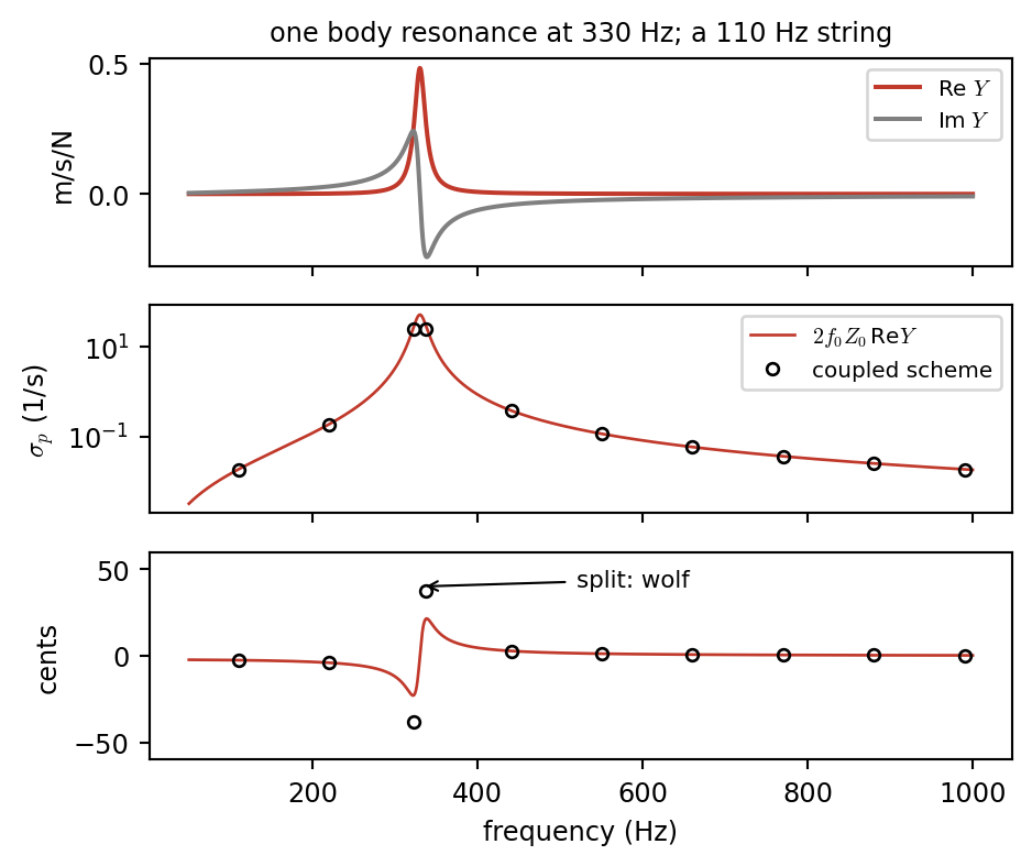
Driving point admittance (mobility): velocity per unit force at the bridge, \[ Y(\omega)=\frac{V(\omega)}{F(\omega)}\quad(\text{m/s/N}) \] End condition \(u_t(L)=Y\cdot\bigl(-Tu_x(L)\bigr)\) with \(u=\sin\beta x\,e^{j\omega t}\): \[ \tan\beta L=jZ_0Y,\qquad Z_0=\sqrt{T\rho A} \] For small \(Z_0Y\): \(\beta L\approx p\pi+jZ_0Y\), so partial \(p\) \[ \begin{aligned} \sigma_p^{\text{bridge}}&=2f_0Z_0\,\mathrm{Re}\,Y(f_p)\\ \Delta f_p&=-\tfrac{f_0}{\pi}\,Z_0\,\mathrm{Im}\,Y(f_p) \end{aligned} \]

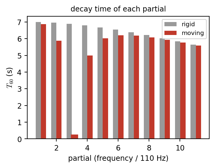
  • \(\mathrm{Re}\,Y>0\): energy leaves the string. Partials near body resonances die fast.
  • Below a resonance (spring-like): flat. Above (mass-like): sharp.
  • Strong coupling: string and body modes split (the cello’s wolf note).
Show code
s = String(f0=110.0, L=0.65, rhoA=3.5e-3, B=0.0)       # lossless, to isolate the bridge
fb, Qb, mb = 330.0, 20, 0.02                           # one body resonance: 330 Hz, Q = 20, 20 g
body1 = Body([fb], [np.pi * fb / Qb], [[1 / np.sqrt(mb)]])
f = np.linspace(50, 1000, 2000); Y = body1.admittance(f)
fp = 110.0 * np.arange(1, 10)
Yp = body1.admittance(fp)
fs_, sg = partials_of(one_step_matrix(s, body1))       # exact: eigenvalues of the coupled scheme
keep = fs_ < 1000; fs_, sg = fs_[keep], sg[keep]
fig, axs = plt.subplots(3, 1, figsize=(5.0, 4.2), sharex=True, height_ratios=[1, 1, 1])
axs[0].plot(f, Y.real, color=COL["bridge"], label="Re $Y$"); axs[0].plot(f, Y.imag, color="0.5", label="Im $Y$")
axs[0].set_ylabel("m/s/N"); axs[0].legend(fontsize=7.5); axs[0].set_title("one body resonance at 330 Hz; a 110 Hz string", fontsize=9)
axs[1].semilogy(f, 2 * 110 * s.Z0 * Y.real, color=COL["bridge"], lw=1, label="$2f_0Z_0\\,$Re$Y$")
axs[1].semilogy(fs_, sg, "ko", ms=4, mfc="none", label="coupled scheme")
axs[1].set_ylabel("$\\sigma_p$ (1/s)"); axs[1].legend(fontsize=7.5)
dfc = lambda f_, df: 1200 * np.log2((f_ + df) / f_)
axs[2].plot(f, dfc(f, -(110 / np.pi) * s.Z0 * Y.imag), color=COL["bridge"], lw=1)
p_ = np.round(fs_ / 110.0)
axs[2].plot(fs_, 1200 * np.log2(fs_ / (110.0 * p_)), "ko", ms=4, mfc="none")
axs[2].set_ylim(-60, 60); axs[2].set_ylabel("cents"); axs[2].set_xlabel("frequency (Hz)")
axs[2].annotate("split: wolf", (330, 40), (520, 40), fontsize=8, arrowprops=dict(arrowstyle="->", lw=0.8))
plt.tight_layout()
plt.show()

The Bridge as a Bank of Oscillators

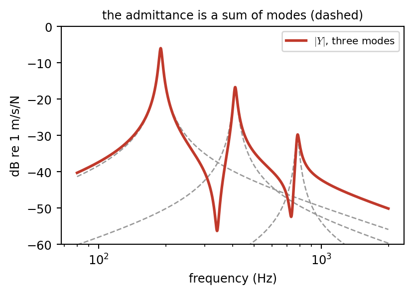
A linear body has modes \((\omega_m,\sigma_m,\phi_m)\) (mass normalized). Seen from the bridge point \(x_b\): \[ Y(\omega)=\sum_m\frac{j\omega\,\phi_m(x_b)^2}{\omega_m^2-\omega^2+2j\sigma_m\omega} \] Time domain: a bank of damped oscillators driven by the bridge force, \[ q_m''+2\sigma_mq_m'+\omega_m^2q_m=-\phi_m(x_b)F,\qquad w=\sum_m\phi_m(x_b)q_m \] Shared force: the string end node keeps its half cell (energy form). Without \(F\), one step gives \(\bar u_N\) and \(\bar w\); with \(F\): \[ u_N^{n+1}=\bar u_N+bF,\quad w^{n+1}=\bar w-GF\ \Rightarrow\ F=\frac{\bar w-\bar u_N}{b+G} \]

ub, qb = s.free(), body.free()
F = (body.phi @ qb - ub[-1]) / (b + body.G)
ub[-1] += b * F;  qn = qb - body.g * body.phi * F

Rigid bridge: \(G=0\), and \(F\) is the reaction force (what we listened to so far).

Show code
body3 = Body([190.0, 410.0, 780.0], 2 * np.pi * np.array([190.0, 410.0, 780.0]) / 60,
             [[1 / np.sqrt(0.05), 1 / np.sqrt(0.08), 1 / np.sqrt(0.2)]])
f = np.logspace(np.log10(80), np.log10(2000), 1500)
fig, ax = plt.subplots(figsize=(4.4, 3.2))
for m in range(3):
    one = Body([body3.om[m] / (2 * np.pi)], [body3.sig[m]], [[body3.phi[0, m]]])
    ax.semilogx(f, 20 * np.log10(np.abs(one.admittance(f))), "--", color="0.6", lw=1)
ax.semilogx(f, 20 * np.log10(np.abs(body3.admittance(f))), color=COL["bridge"], lw=2, label="$|Y|$, three modes")
ax.set_xlabel("frequency (Hz)"); ax.set_ylabel("dB re 1 m/s/N"); ax.set_ylim(-60, 0)
ax.set_title("the admittance is a sum of modes (dashed)", fontsize=9); ax.legend(fontsize=7.5)
plt.tight_layout()
plt.show()

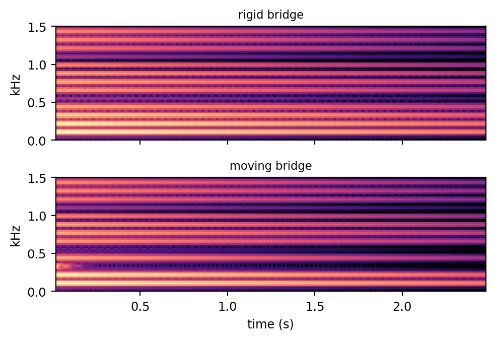
Rigid vs Moving Bridge

Show code
fig, axs = plt.subplots(2, 1, figsize=(5.2, 3.6), sharex=True)
for ax, (name, (y, _, _)) in zip(axs, bridge_runs.items()):
    show_spec(ax, y, f"{name} bridge", fmax=1.5)
    ax.set_ylabel("kHz")
axs[1].set_xlabel("time (s)")
plt.tight_layout()
plt.show()

Show code
fig, ax = plt.subplots(figsize=(3.8, 3.0))
for (name, (_, f_, sg_)), col, off in zip(bridge_runs.items(), ["0.6", COL["bridge"]], [-0.17, 0.17]):
    keep = f_ < 1250
    ax.bar(f_[keep] / 110 + off, 3 * np.log(10) / sg_[keep], width=0.34, color=col, label=name)
ax.set_xlabel("partial (frequency / 110 Hz)"); ax.set_ylabel("$T_{60}$ (s)")
ax.set_title("decay time of each partial", fontsize=9); ax.legend(fontsize=7.5)
plt.tight_layout()
plt.show()

rigid bridge

moving bridge (resonance at the 3rd partial)

Sympathetic Resonance in Bridges

Multiple Strings on One Bridge

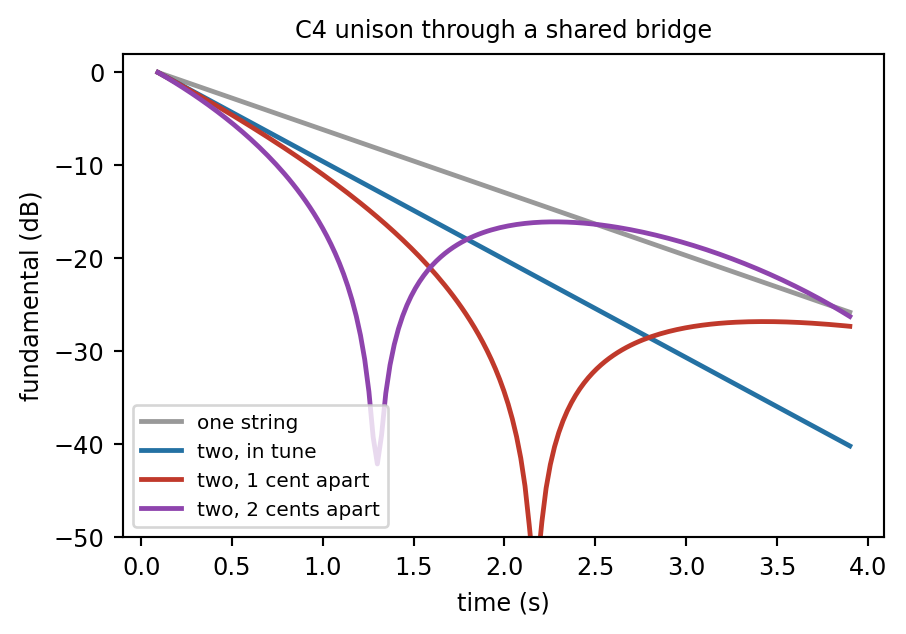
\(P\) strings on one bridge: \(P\) end conditions, one \(P\times P\) solve, constant in time: \[ \begin{aligned} \bigl(\operatorname{diag}(b_p)+\mathbf{G}\bigr)\mathbf{F}&=\bar{\mathbf{w}}-\bar{\mathbf{u}}_N\\ G_{pq}&=\textstyle\sum_mg_m\phi_m(x_p)\phi_m(x_q) \end{aligned} \]

  • In phase strings push the bridge together: twice the energy loss.
  • Out of phase forces cancel at the bridge: almost no loss.
  • Slight mistuning turns the first into the second: a fast first stage, then a long aftersound (two-stage decay).
  • Same equations: sympathetic strings (sitar, viola d’amore, piano with the pedal down), attached at different points.
Show code
fig, ax = plt.subplots(figsize=(4.8, 3.4))
win, hop = 8192, 1024
for (name, y), col in zip(unisons.items(), ["0.6", COL["string"], COL["bridge"], COL["exciter"]]):
    b0 = int(round(261.6 * win / fs))                              # the fundamental's bin
    env = np.array([np.abs(np.fft.rfft(y[i:i + win] * np.hanning(win)))[b0 - 2:b0 + 3].max()
                    for i in range(0, len(y) - win, hop)])
    ax.plot((np.arange(len(env)) * hop + win / 2) / fs, 20 * np.log10(env / env.max()), color=col, lw=1.8, label=name)
ax.set_xlabel("time (s)"); ax.set_ylabel("fundamental (dB)"); ax.set_ylim(-50, 2)
ax.set_title("C4 unison through a shared bridge", fontsize=9); ax.legend(fontsize=7.5, loc="lower left")
plt.tight_layout()
plt.show()

one string

two strings, in tune

two strings, 2 cents apart

Finite Elements for the Body

Why Finite Elements?

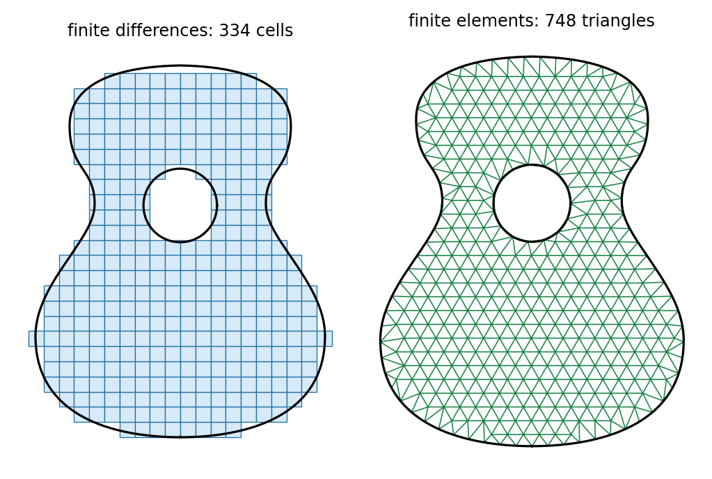
Finite differences need a box grid:

  • curved rim, sound hole: a staircase;
  • boundary conditions on curves are awkward;
  • no local refinement.

Finite elements split the domain into triangles:

  • the mesh follows the shape, sizes can vary;
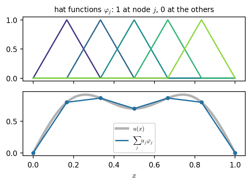
  • unknowns: values at the vertices, \(u_h=\sum_ju_j\varphi_j\) with hat functions \(\varphi_j\);
  • start from the weak (integral) form: matrices \(\mathbf{K}\), \(\mathbf{M}\), then the same eigenproblem as the marimba.

The cotangent Laplacian of graphics is exactly this \(\mathbf{K}\) (class 14 map).

Show code
outline = guitar_outline(); hole = circle(*HOLE, 0.004)
fig, axs = plt.subplots(1, 2, figsize=(5.4, 4.0))
hc = 0.02                                                # a coarse box grid, cells kept if their center is inside
X, Y = np.meshgrid(np.arange(-0.2, 0.2, hc) + hc / 2, np.arange(0, 0.5, hc) + hc / 2)
C = np.c_[X.ravel(), Y.ravel()]
inside = Path(outline).contains_points(C) & ~Path(hole).contains_points(C)
for cx, cy in C[inside]:
    axs[0].add_patch(plt.Rectangle((cx - hc / 2, cy - hc / 2), hc, hc, fc="#d6eaf8", ec=COL["string"], lw=0.5))
pts_c, tri_c, _ = mesh_domain(outline, [hole], h=0.02)
axs[1].triplot(pts_c[:, 0], pts_c[:, 1], tri_c, color=COL["body"], lw=0.6)
for ax, title in zip(axs, [f"finite differences: {inside.sum()} cells", f"finite elements: {len(tri_c)} triangles"]):
    ax.plot(*np.r_[outline, outline[:1]].T, color="k", lw=1.2); ax.plot(*np.r_[hole, hole[:1]].T, color="k", lw=1.2)
    ax.set_aspect("equal"); ax.axis("off"); ax.set_title(title, fontsize=9)
plt.tight_layout()
plt.show()
1D Galerkin: Hat Functions and Element Matrices

Weak form: multiply \(\rho Au_{tt}=Tu_{xx}\) by a test function \(v\) and integrate by parts: \[ \int_0^L\rho A\,u_{tt}\,v\,dx+\int_0^LT\,u_x\,v_x\,dx=0\quad\forall v \] Galerkin: \(u\approx\sum_ju_j(t)\varphi_j(x)\) and \(v=\varphi_i\): \[ \mathbf{M}\mathbf{u}''=-\mathbf{K}\mathbf{u},\qquad M_{ij}=\int\rho A\,\varphi_i\varphi_j,\quad K_{ij}=\int T\varphi_i'\varphi_j' \] Element by element (length \(h\)), then assemble: \[ \mathbf{K}_e=\frac{T}{h}\begin{bmatrix}1&-1\\-1&1\end{bmatrix},\qquad \mathbf{M}_e=\frac{\rho Ah}{6}\begin{bmatrix}2&1\\1&2\end{bmatrix} \]

for e in range(N):                       # element e joins nodes e, e+1
    idx = np.ix_([e, e + 1], [e, e + 1])
    K[idx] += T / h * np.array([[1, -1], [-1, 1]])
    M[idx] += rhoA * h / 6 * np.array([[2, 1], [1, 2]])

Interior rows: \(\mathbf{K}\to\frac{T}{h}(-1,2,-1)\), the class 14 \(\delta_{xx}\); \(\ \mathbf{M}\to\frac{\rho Ah}{6}(1,4,1)\), consistent mass.

Show code
xn = np.linspace(0, 1, 7); xf = np.linspace(0, 1, 600)
hat = lambda j: np.interp(xf, xn, np.eye(len(xn))[j])                 # piecewise linear, 1 at node j
uj = np.sin(np.pi * xn) + 0.3 * np.sin(3 * np.pi * xn)
fig, axs = plt.subplots(2, 1, figsize=(4.4, 3.3), sharex=True)
for j in range(1, 6):
    axs[0].plot(xf, hat(j), color=plt.cm.viridis(j / 6), lw=1.6)
axs[0].set_title("hat functions $\\varphi_j$: 1 at node $j$, 0 at the others", fontsize=9)
axs[1].plot(xf, np.sin(np.pi * xf) + 0.3 * np.sin(3 * np.pi * xf), color="0.7", lw=3, label="$u(x)$")
axs[1].plot(xf, sum(uj[j] * hat(j) for j in range(7)), color=COL["string"], lw=1.6, label="$\\sum_j u_j\\varphi_j$")
axs[1].plot(xn, uj, "o", color=COL["string"], ms=4)
axs[1].legend(fontsize=7.5); axs[1].set_xlabel("$x$")
plt.tight_layout()
plt.show()

Consistent vs Lumped Mass

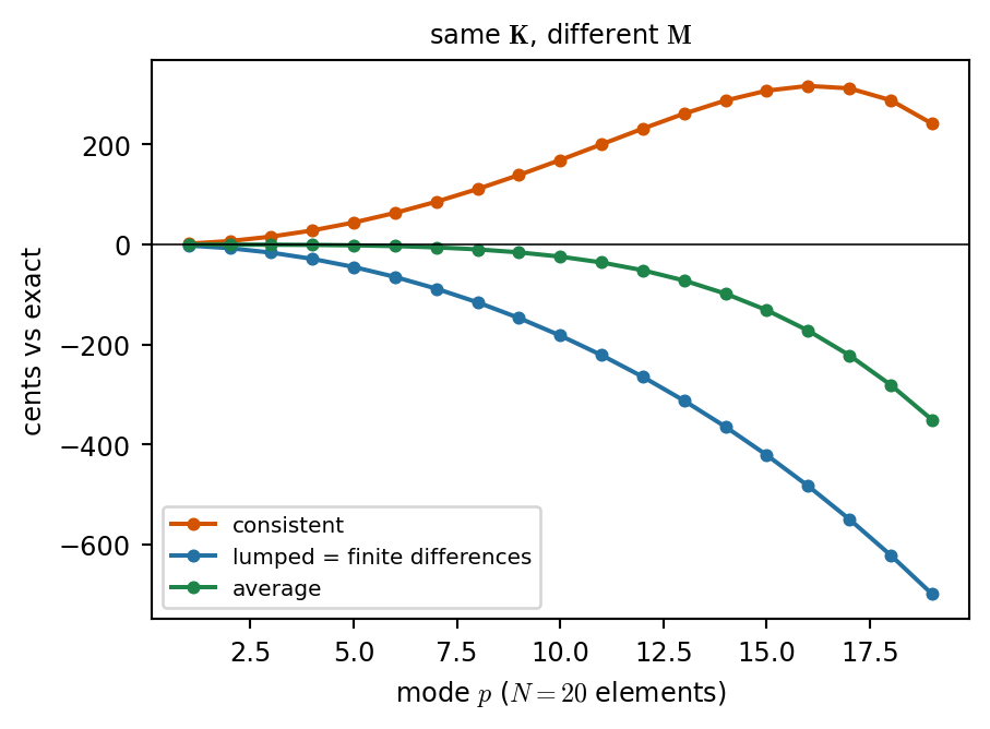
Fixed ends: sines are exact eigenvectors, so read \(\omega\) off the symbols (\(s=\sin\frac{\beta h}{2}\)):

mass \(\omega^2\) error
lumped \(\rho Ah\,\mathbf{I}\) \(\frac{4c^2}{h^2}s^2\) \(-\frac{(\beta h)^2}{24}\)
consistent \((1,4,1)\) \(\frac{4c^2}{h^2}\frac{s^2}{1-\frac23s^2}\) \(+\frac{(\beta h)^2}{24}\)
average \(\frac{4c^2}{h^2}\frac{s^2}{1-\frac13s^2}\) \(O((\beta h)^4)\)
  • Lumped mass FEM = finite differences (class 14): flat.
  • Consistent: sharp, an upper bound (Rayleigh-Ritz).
  • Time stepping: lumped is diagonal, so explicit (and exact at \(\lambda=1\)); consistent needs a tridiagonal solve per step.
  • For the body we only need modes, so consistent mass is fine.
Show code
N, c = 20, 1.0; h = 1 / N
K = np.zeros((N + 1, N + 1)); Mc = np.zeros_like(K)
for e in range(N):
    idx = np.ix_([e, e + 1], [e, e + 1])
    K[idx] += c**2 / h * np.array([[1, -1], [-1, 1]])
    Mc[idx] += h / 6 * np.array([[2, 1], [1, 2]])
Ml = np.diag(Mc.sum(1))                                 # lumped: row sums on the diagonal
K, Mc, Ml = K[1:-1, 1:-1], Mc[1:-1, 1:-1], Ml[1:-1, 1:-1]   # fixed ends
exact = c * np.pi * np.arange(1, N)
fig, ax = plt.subplots(figsize=(4.8, 3.6))
for M_, col, lab in [(Mc, COL["stiff"], "consistent"), (Ml, COL["string"], "lumped = finite differences"),
                     ((Mc + Ml) / 2, COL["body"], "average")]:
    om = np.sqrt(sla.eigh(K, M_, eigvals_only=True))
    ax.plot(np.arange(1, N), 1200 * np.log2(om / exact), "o-", color=col, ms=3.5, label=lab)
ax.axhline(0, color="k", lw=0.6)
ax.set_xlabel("mode $p$ ($N=20$ elements)"); ax.set_ylabel("cents vs exact")
ax.set_title("same $\\mathbf{K}$, different $\\mathbf{M}$", fontsize=9); ax.legend(fontsize=7.5)
plt.tight_layout()
plt.show()

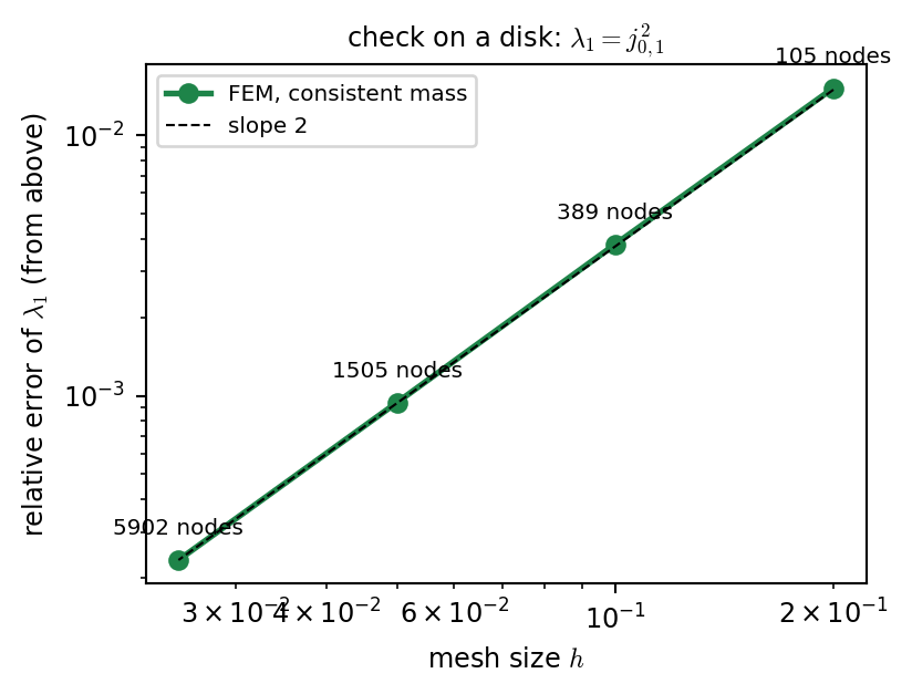
2D: Linear Triangles

Weak form of the membrane: \(\int\rho H\,u_{tt}v+\int T\,\nabla u\cdot\nabla v=0\).

On a triangle of area \(A\) the hats are the barycentric coordinates \(\lambda_i\), with constant gradients: \[ K^e_{ij}=A\,\nabla\lambda_i\cdot\nabla\lambda_j,\qquad M^e_{ij}=\frac{A}{12}(1+\delta_{ij}) \] \(\nabla\lambda_i\): the opposite edge rotated by \(90^\circ\), over \(2A\).

grad = np.stack([-e[..., 1], e[..., 0]], -1) / (2 * area[:, None, None])
Ke = area[:, None, None] * np.einsum("tid,tjd->tij", grad, grad)
Me = area[:, None, None] / 12 * (np.ones((3, 3)) + np.eye(3))
I, J = np.repeat(tri, 3, axis=1).ravel(), np.tile(tri, (1, 3)).ravel()
K = sp.coo_matrix((Ke.ravel(), (I, J))).tocsr()   # duplicates add up:
M = sp.coo_matrix((Me.ravel(), (I, J))).tocsr()   # that is assembly

Mesh with scipy only: points on the boundary every \(h\), a hexagonal lattice inside, Delaunay, drop the triangles outside.

Show code
hs, err, nodes = [0.2, 0.1, 0.05, 0.025], [], []
exact = jn_zeros(0, 1)[0]**2                            # unit disk, fixed rim: j_01^2
for h in hs:
    pts, tri, bnd = mesh_domain(circle(0, 0, 1, h / 4), h=h)
    K, M = p1_matrices(pts, tri)
    free = np.setdiff1d(np.arange(len(pts)), bnd)
    lam1 = spla.eigsh(K[free][:, free], 1, M[free][:, free], sigma=0)[0][0]
    err.append((lam1 - exact) / exact); nodes.append(len(pts))
fig, ax = plt.subplots(figsize=(4.4, 3.4))
ax.loglog(hs, err, "o-", color=COL["body"], lw=2, label="FEM, consistent mass")
ax.loglog(hs, err[-1] * (np.array(hs) / hs[-1])**2, "k--", lw=0.8, label="slope 2")
for h, e, n in zip(hs, err, nodes):
    ax.text(h, e * 1.25, f"{n} nodes", fontsize=7.5, ha="center")
ax.set_xlabel("mesh size $h$"); ax.set_ylabel("relative error of $\\lambda_1$ (from above)")
ax.set_title("check on a disk: $\\lambda_1=j_{0,1}^2$", fontsize=9); ax.legend(fontsize=7.5)
plt.tight_layout()
plt.show()

Modes of a Guitar Top

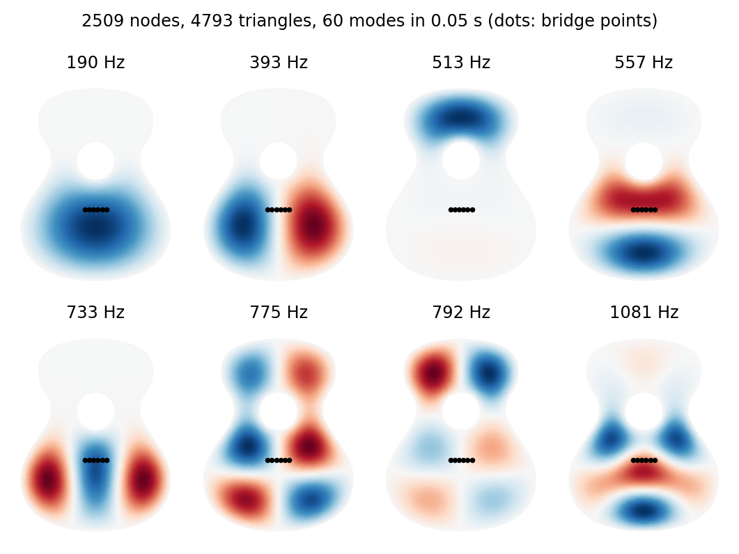
Model (state it)

Uniform, isotropic, unbraced top; Navier edges \(u=\nabla^2u=0\) on the rim and around the reinforced sound hole. Then the plate modes equal the membrane modes, \[ -\nabla^2\phi_m=\mu_m\phi_m\ \Rightarrow\ \nabla^4\phi_m=\mu_m^2\phi_m, \] with plate frequencies \(\omega_m=\kappa\mu_m\). \(\kappa\) is set so that mode 1 is at 190 Hz (braces stiffen a real top).

Not modeled: orthotropic spruce, braces, the air cavity (the Helmholtz mode near 100 Hz). Real tops need plate or shell elements.

Outline, sound hole and saddle: traced from a CC0 drawing of an acoustic guitar, scaled to a 49 cm body.

lam, V = spla.eigsh(K_f, 60, rhoH * M_f, sigma=0)
f_m = kappa * lam / (2 * np.pi)
Show code
rhoH = 450 * 2.8e-3                                     # spruce, 2.8 mm: areal density (kg/m^2)
t0 = time.perf_counter()
pts, tri, bnd = mesh_domain(guitar_outline(), [circle(*HOLE, 0.004)], h=0.008)
Kg, Mg = p1_matrices(pts, tri)
free = np.setdiff1d(np.arange(len(pts)), bnd)
lam, V = spla.eigsh(Kg[free][:, free], 60, rhoH * Mg[free][:, free], sigma=0)
o = np.argsort(lam); lam, V = lam[o], V[:, o]
kappa_p = 2 * np.pi * 190.0 / lam[0]                   # plate: omega = kappa mu
t_fem = time.perf_counter() - t0
f_m = kappa_p * lam / (2 * np.pi)
Phi = np.zeros((len(pts), len(lam))); Phi[free] = V     # mass normalized: Phi^T (rhoH M) Phi = I
fig, axs = plt.subplots(2, 4, figsize=(5.6, 4.3))
for m, ax in enumerate(axs.flat):
    v = Phi[:, m]; a = np.abs(v).max()
    ax.tripcolor(pts[:, 0], pts[:, 1], tri, v, cmap="RdBu_r", shading="gouraud", vmin=-a, vmax=a)
    ax.plot(BRIDGE_X, np.full(6, BRIDGE_Y), "o", color="k", ms=1.8)
    ax.set_aspect("equal"); ax.axis("off"); ax.set_title(f"{f_m[m]:.0f} Hz", fontsize=9)
fig.suptitle(f"{len(pts)} nodes, {len(tri)} triangles, 60 modes in {t_fem:.2f} s (dots: bridge points)", fontsize=9)
plt.tight_layout()
plt.show()
Admittance at the Bridge

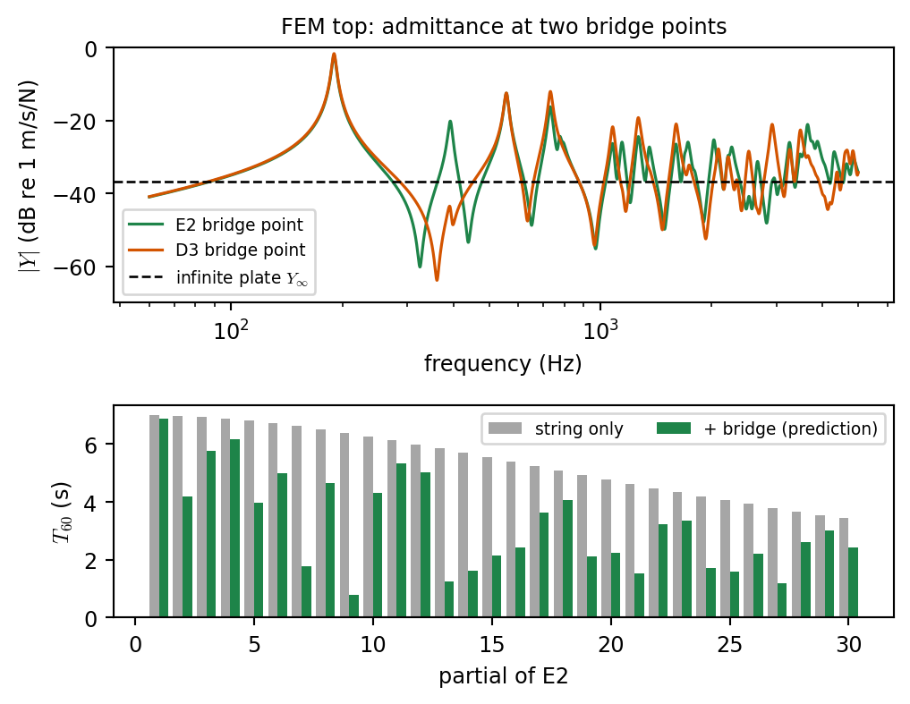
Bridge point values: barycentric weights of the triangle that contains \(x_b\), i.e. the FEM interpolation \(I\) (and \(J=I^\top\) for the force). \[ \phi_m(x_b)=\sum_{i\in\text{tri}}\lambda_i(x_b)\,\Phi_{im} \] Damping: \(Q=40\) per mode, \(\sigma_m=\omega_m/(2Q)\).

Sanity check: at high frequency the modal sum hovers around the infinite plate value \[ Y_\infty=\frac{1}{8\kappa\rho H} \] Prediction for each partial of the low E string: \[ \sigma_p=\sigma_{\text{string}}(f_p)+2f_0Z_0\,\mathrm{Re}\,Y(f_p) \]

Show code
f = np.logspace(np.log10(60), np.log10(5000), 3000)
fig, axs = plt.subplots(2, 1, figsize=(5.4, 4.2), height_ratios=[1.2, 1])
for p, col in [(0, COL["body"]), (2, COL["stiff"])]:
    axs[0].semilogx(f, 20 * np.log10(np.abs(guitar.admittance(f, p))), color=col, lw=1.2,
                    label=f"{['E2', 'A2', 'D3', 'G3', 'B3', 'E4'][p]} bridge point")
axs[0].axhline(20 * np.log10(Y_inf), color="k", ls="--", lw=1, label="infinite plate $Y_\\infty$")
axs[0].set_ylabel("$|Y|$ (dB re 1 m/s/N)"); axs[0].set_ylim(-70, 0); axs[0].legend(fontsize=7, loc="lower left")
axs[0].set_xlabel("frequency (Hz)"); axs[0].set_title("FEM top: admittance at two bridge points", fontsize=9)
s = guitar_string(0)
fp, sig_s = (v[:30] for v in partials_of(one_step_matrix(s)))   # the string alone (rigid bridge), scheme partials
sig_pred = sig_s + 2 * s.f0 * s.Z0 * guitar.admittance(fp, 0).real
axs[1].bar(np.arange(1, 31) - 0.2, 3 * np.log(10) / sig_s, 0.4, color="0.65", label="string only")
axs[1].bar(np.arange(1, 31) + 0.2, 3 * np.log(10) / sig_pred, 0.4, color=COL["body"], label="+ bridge (prediction)")
axs[1].set_xlabel("partial of E2"); axs[1].set_ylabel("$T_{60}$ (s)"); axs[1].legend(fontsize=7, ncol=2)
plt.tight_layout()
plt.show()
Putting It Together

One Time Step of the Whole Instrument

for n in range(n_out):
    ub = s.free()                              # 1 string, explicit
    exciter.apply(n, s, ub)                    # 2 exciter (Newton for a bow)
    qb = body.free()                           # 3 body modes
    F = (body.phi @ qb - ub[-1]) / (b + body.G)  # 4 shared force
    ub[-1] += b * F
    qn = qb - body.g * body.phi * F
    y[n] = A @ (qn - 2*body.q + body.qp) / k**2  # 5 radiation
    s.commit(ub); body.commit(qn)

Radiation proxy: at low frequency the top is a small loudspeaker; the pressure follows its volume acceleration \[ p(t)\propto\frac{d^2}{dt^2}\int_{\text{top}}u\,dA=\sum_mA_m\,q_m'',\qquad A_m=\int\phi_m\,dA \] Symmetric modes (\(A_m\) large) radiate; dipoles (\(A_m\approx0\)) barely do.

Work per audio sample (low E string + FEM top):

part operations
string, \(N\approx200\) \(\approx20N\)
exciter \(O(1)\), Newton: \(\approx3\) iterations
body, \(60\) modes \(\approx6\times60\)
bridge one division

The body costs less than the string. Six strings with sympathetic coupling: a \(6\times6\) matrix inverted once.

Same pattern everywhere

explicit free updates, then a small solve for the shared forces.

Hear the Progression

Show code
fig, axs = plt.subplots(1, 4, figsize=(10, 2.5), sharey=True)
for i, (ax, (name, y)) in enumerate(zip(axs, prog.items())):
    show_spec(ax, y, f"{i + 1}. {name}", fmax=3)
    ax.set_xlabel("time (s)")
axs[0].set_ylabel("kHz")
plt.tight_layout()
plt.show()
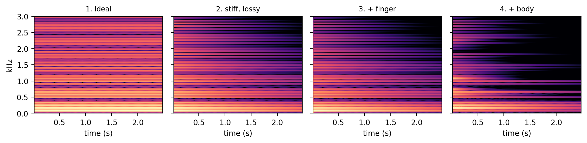
1. ideal string (class 14)

2. stiff, lossy (class 15)

3. + finger force

4. + FEM body, two-way

One-Way or Two-Way Coupling?

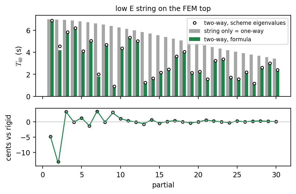
One-way: rigid bridge force \(\ast\) body impulse response (a convolution; commuted synthesis, class 18).

  • the string never feels the body;
  • partial decay times stay those of a rigid bridge.

Two-way: shared force at every step.

  • energy flows into the body: each partial gets its own decay and a small detuning;
  • costs the modal bank (cheap, previous slide).

Check: the scheme is linear, \(\mathbf{x}^{n+1}=\mathbf{A}\mathbf{x}^n\). Its eigenvalues \(z\) give every partial exactly: \(f=\frac{\angle z}{2\pi k}\), \(\sigma=-\frac{\ln|z|}{k}\).

Show code
p = np.arange(1, 31)
fig, axs = plt.subplots(2, 1, figsize=(5.4, 3.6), sharex=True, height_ratios=[1.4, 1])
near = lambda f_: np.nonzero(np.abs(f_two - f_) < 0.4 * 82.41)[0]   # coupled modes near each string partial:
pick = np.array([c_[np.argmin(sg_two[c_])] for c_ in map(near, fp)]) # keep the least damped (string-like) one
axs[0].bar(p - 0.2, 3 * np.log(10) / sig_s, 0.4, color="0.65", label="string only = one-way")
axs[0].bar(p + 0.2, 3 * np.log(10) / sig_pred, 0.4, color=COL["body"], label="two-way, formula")
axs[0].plot(p + 0.2, 3 * np.log(10) / sg_two[pick], "ko", ms=3.5, mfc="white", label="two-way, scheme eigenvalues")
axs[0].set_ylabel("$T_{60}$ (s)"); axs[0].legend(fontsize=7, ncol=1, loc="upper right")
axs[0].set_title("low E string on the FEM top", fontsize=9)
axs[1].plot(p, 1200 * np.log2(f_two[pick] / fp), "ko", ms=3.5, mfc="white")
axs[1].plot(p, 1200 * np.log2((fp - 82.41 / np.pi * s.Z0 * guitar.admittance(fp, 0).imag) / fp), "-", color=COL["body"], lw=1.2)
axs[1].axhline(0, color="0.7", lw=0.6); axs[1].set_ylabel("cents vs rigid"); axs[1].set_xlabel("partial")
plt.tight_layout()
plt.show()
one-way (filtered through the body)

two-way (coupled)

Virtual Guitar Demo

Stability and Cost

Energy-Neutral Coupling

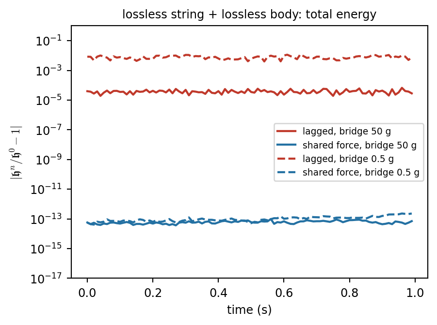
Each part has a discrete energy, non-negative under its own stability condition (classes 13 to 15). Coupled: \[ \begin{aligned} \delta_{t+}\mathfrak{h}_{\text{string}}&=-\text{loss}+F\,\delta_{t\cdot}u_N\\ \delta_{t+}\mathfrak{h}_{\text{body}}&=-\text{loss}-F\,\delta_{t\cdot}w \end{aligned} \] Same \(F\) and \(u_N=w\) at every step \(\Rightarrow\) the coupling terms cancel: \[ \delta_{t+}\bigl(\mathfrak{h}_{\text{string}}+\mathfrak{h}_{\text{body}}\bigr)=-\text{loss}\le0 \]

  • Stability of the whole = stability of the parts: no new CFL condition.
  • A lagged coupling (string follows the body, body pushed by last step’s slope) breaks the cancellation; worse for light bridges (a violin bridge is about 2 g).
Show code
def coupled_energy(mb, lagged, dur=1.0):
    s = String(f0=110.0, L=0.65, rhoA=3.5e-3, B=1e-4); pluck_ic(s, 0.2)
    bd = Body([180.0], [0.0], [[1 / np.sqrt(mb)]])       # lossless body
    b, E = s.gain[-1], []
    for n in range(int(dur * fs)):
        ub, qb = s.free(), bd.free()
        if not lagged:                                    # shared force
            F = (bd.phi[0] @ qb - ub[-1]) / (b + bd.G[0, 0])
            qn = qb - bd.g * bd.phi[0] * F; ub[-1] += b * F
        else:                                             # lagged
            Fs = s.T * (s.u[-2] - s.u[-1]) / s.h
            qn = qb + bd.g * bd.phi[0] * Fs; ub[-1] = bd.phi[0] @ qn
        E.append(s.energy(ub) + bd.energy(qn)); s.commit(ub); bd.commit(qn)
    E = np.abs(np.array(E) / E[0] - 1) + 1e-17
    return E.reshape(-1, 441).max(1)                      # largest deviation in each 10 ms block
fig, ax = plt.subplots(figsize=(4.8, 3.6))
t = np.arange(100) * 0.01
for mb, ls in [(0.05, "-"), (5e-4, "--")]:
    ax.semilogy(t, coupled_energy(mb, True), ls, color=COL["bridge"], lw=1.6, label=f"lagged, bridge {1e3 * mb:g} g")
    ax.semilogy(t, coupled_energy(mb, False), ls, color=COL["string"], lw=1.6, label=f"shared force, bridge {1e3 * mb:g} g")
ax.set_xlabel("time (s)"); ax.set_ylabel("$|\\mathfrak{h}^n/\\mathfrak{h}^0-1|$"); ax.set_ylim(1e-17, 1)
ax.set_title("lossless string + lossless body: total energy", fontsize=9); ax.legend(fontsize=7, loc="center right")
plt.tight_layout()
plt.show()
Couplings That Change the Stability Condition

A spring \(K_s\) at one point of the string (a prepared string):

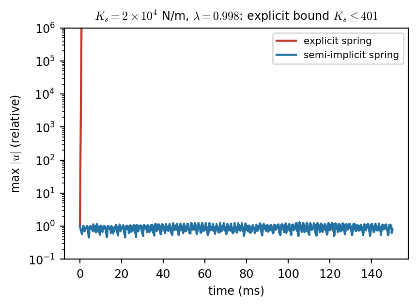
  • explicit \(F=-K_s\,u_p^n\): the energy needs \[ K_s\,k^2\le4\rho Ah\,(1-\lambda^2) \] at \(\lambda\to1\) (most accurate) nothing is allowed.
  • semi-implicit \(F=-K_s\,\frac{u_p^{n+1}+u_p^{n-1}}{2}\): one division, the spring energy is always \(\ge0\), no condition.
connection scheme extra condition
bridge, shared force implicit, 1 scalar none
spring explicit \(K_sk^2\le4\rho Ah(1-\lambda^2)\)
spring, damper semi-implicit none
hammer explicit none (may ring near the limit)
bow implicit, Newton unique if \(cF_B\max(-\phi')<1\)
Show code
def spring_run(Ks, semi, dur=0.15):
    s = String(f0=110.0, L=0.65, rhoA=3.5e-3, B=0.0); pluck_ic(s, 0.2)
    p, amp = int(0.37 * s.N), []
    g = s.gain[p]
    for n in range(int(dur * fs)):
        ub = s.free()
        if semi:
            ub[p] = (ub[p] - g * Ks * s.up[p] / 2) / (1 + g * Ks / 2)
        else:
            ub[p] += -g * Ks * s.u[p]
        ub[-1] = 0.0; s.commit(ub)
        amp.append(np.abs(s.u).max())
        if not np.isfinite(amp[-1]) or amp[-1] > 1e3: break
    lam = 2 * s.L * s.f0 * k / s.h
    return np.array(amp), 4 * s.rhoA * s.h * (1 - lam**2) / k**2, lam
fig, ax = plt.subplots(figsize=(4.6, 3.4))
for semi, col in [(False, COL["bridge"]), (True, COL["string"])]:
    a, bound, lam = spring_run(2e4, semi)
    ax.semilogy(1e3 * np.arange(len(a)) * k, a / a[0], color=col, lw=1.6,
                label=("semi-implicit" if semi else "explicit") + " spring")
ax.set_xlabel("time (ms)"); ax.set_ylabel("max $|u|$ (relative)"); ax.set_ylim(0.1, 1e6)
ax.set_title(f"$K_s=2\\times10^4$ N/m, $\\lambda={lam:.3f}$: explicit bound $K_s\\leq{bound:.0f}$", fontsize=9)
ax.legend(fontsize=7.5)
plt.tight_layout()
plt.show()
Preparing a String: Springs and Dampers

Show code
fig, axs = plt.subplots(1, 3, figsize=(9.6, 2.6), sharey=True)
for ax, (name, y), col in zip(axs, preps.items(), ["0.4", COL["exciter"], COL["string"]]):
    seg = y[int(0.3 * fs):int(1.3 * fs)]                  # a second of the sustained part
    Y = np.abs(np.fft.rfft(seg * np.hanning(len(seg)))); f = np.fft.rfftfreq(len(seg), k)
    for m in range(1, 13):
        ax.axvline(m, color="0.85", ls="--", lw=0.7, zorder=0)
    ax.plot(f / 110, 20 * np.log10(Y / Y.max() + 1e-9), color=col, lw=0.8)
    ax.set_xlim(0, 12.5); ax.set_ylim(-70, 3); ax.set_title(f"A2 string, {name}", fontsize=9)
    ax.set_xlabel("frequency / 110 Hz (dashed: harmonics)")
axs[0].set_ylabel("dB (0.3 to 1.3 s)")
plt.tight_layout()
plt.show()
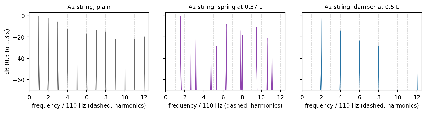
plain

spring \(2\times10^4\) N/m at \(0.37L\): inharmonic

damper at \(0.5L\): odd partials die, an octave remains

Cost: Precompute Once, Pay per Sample

cost note
FEM precompute (mesh + 60 modes) 0.05 s once 2509 nodes
string, low E \(\approx3980\) ops/sample \(N=199\)
modal body \(\approx360\) ops/sample 60 modes up to 5.9 kHz
bridge 1 division/sample
FEM mesh stepped directly (explicit) \(\approx23\times2284\times7\) ops/sample \(\omega_{\max}k=46\): 23 substeps
FD plate at 44.1 kHz (class 15) \(\approx226\times13\) ops/sample \(h=2.5\) cm: coarse, staircase
this Python loop 0.56 s per second of audio (numpy overhead dominates)

Choosing

Linear and irregular (bodies, soundboards): FEM modes once, modal bank per sample. Nonlinear or in contact (strings under a bow, hammers): finite differences and lumped models in time. Glue: shared forces, solved as small systems.

Beyond Linear Strings

Tension Modulation: Pitch Glides

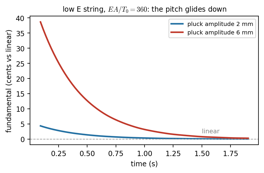
A large pluck stretches the string; the tension rises with the amplitude (Kirchhoff-Carrier): \[ \rho A\,u_{tt}=\Bigl(T_0+\frac{EA}{2L}\int_0^Lu_x^2\,dx\Bigr)u_{xx} \] Higher tension, higher pitch; as the sound decays the pitch glides down.

  • One scalar \(T^n\) per step (here explicit; energy conserving versions solve a rank one system).
  • Higher tension = faster waves: leave CFL headroom (here 20%; without it the run blows up).
  • Phantom partials (piano bass): nonlinear coupling to longitudinal waves creates sums \(f_p+f_q\) of partials. A richer model than this one.
Show code
fig, ax = plt.subplots(figsize=(4.8, 3.2))
t_, ref = pitch_track(kc_lin, 82.41)
for a, col in [(2, COL["string"]), (6, COL["bridge"])]:
    t_, fr = pitch_track(kc[a], 82.41)
    ax.plot(t_, 1200 * np.log2(fr / ref), color=col, lw=2, label=f"pluck amplitude {a} mm")
ax.axhline(0, color="0.6", lw=0.8, ls="--"); ax.text(1.5, 2, "linear", color="0.5", fontsize=8)
ax.set_xlabel("time (s)"); ax.set_ylabel("fundamental (cents vs linear)")
ax.set_title("low E string, $EA/T_0=360$: the pitch glides down", fontsize=9); ax.legend(fontsize=7.5)
plt.tight_layout()
plt.show()
linear, 6 mm

tension modulated, 6 mm

Looking Ahead

Where These Ideas Come Back

  • Percussive Instruments and Modal Synthesis (next class): today’s FEM modes and modal oscillator banks become the whole instrument (bells, gongs, bars); mallets are today’s hammer.
  • Wind Instruments and Digital Waveguides: the reed is a lumped nonlinearity solved once per step like the bow, coupled to the bore by a shared pressure and flow; one-way (commuted) synthesis of strings and bodies with waveguides.
  • Sound Effects: squeaks are bow friction, rattles are two-sided contacts, impacts are hammers.
  • Projects: a heritage string instrument, e.g. the gayageum (silk strings over movable bridges, a paulownia body) or the geomungo (struck with a stick): exciter, string, bridge, FEM body, and pitch bends (nonghyeon) as tension changes.

Recap

Recap on Today’s ILO

  • Exciters: spread with \(J\), read with \(I=J^\top\); explicit string, then one scalar equation at the contact (hammer: closed form; bow: Newton, nearest root when not unique).
  • Bridge: admittance \(Y\); partials decay by \(2f_0Z_0\,\mathrm{Re}\,Y\) and shift by \(-\frac{f_0}{\pi}Z_0\,\mathrm{Im}\,Y\); in time, a modal bank + one shared force; shared bridges give double decay and sympathetic strings.
  • FEM: weak form, element matrices, assembly; lumped mass = finite differences, consistent mass bounds from above; guitar top modes and the bridge admittance.
  • Stability and cost: shared forces are energy neutral (no new CFL condition); explicit springs are not. FEM once, the string dominates the per-sample cost.
  • Nonlinear: tension modulation glides the pitch; leave CFL headroom.