Percussive Instruments and Modal Synthesis


Topics in Digital Heritage:
Numerical Methods for Digital Reconstruction

Jin Woo Lee

KAIST

Fall 2026

Recap

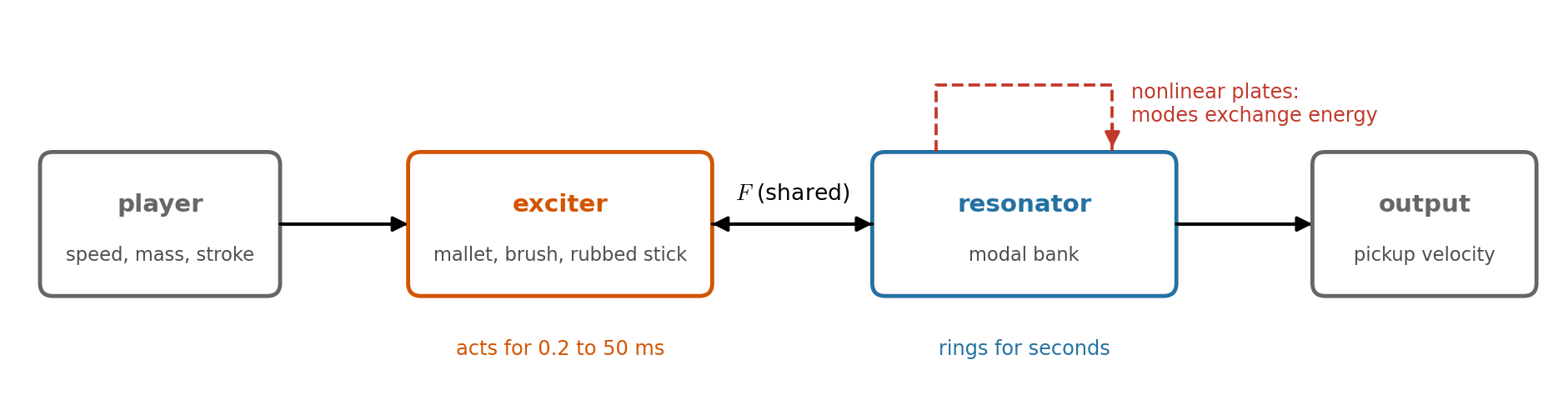
Last Time: Exciter, Resonator, Shared Force

  • Coupled parts: exciter and resonator share one force \(F\) (class 16)
  • Body = modal bank, modes from FEM (class 16)
  • Carved bar modes from \(\mathbf{K}\mathbf{v}=\omega^2\mathbf{M}\mathbf{v}\) (class 15)
  • Exact recursion and mallet contact (class 13, contact)
  • Bow friction: one Newton solve per step (class 16)

Today: percussion is the home of modal synthesis, until the plate goes nonlinear.

Show code
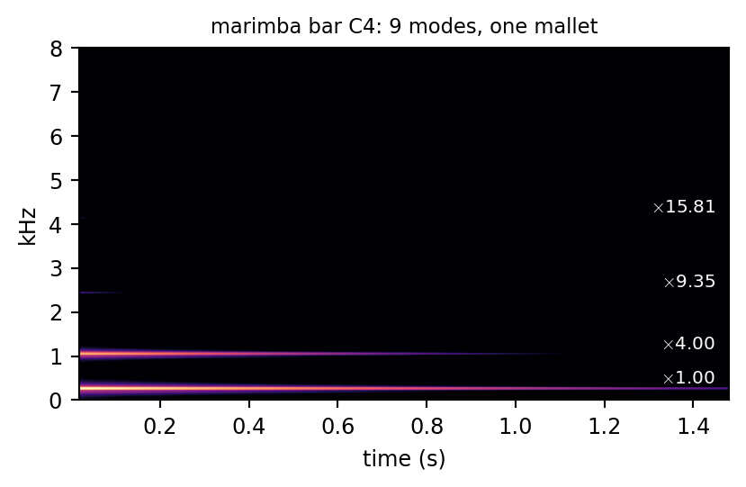
md, pe, po = bar_instrument(261.6, ratio=4)           # the class 15 marimba bar, C4
r = strike(md, pe, po, MH=0.03, KH=1e10, vH=1.5, dur=1.5, scheme="explicit")
save_wav("recap_marimba", r["y"])
fig, ax = plt.subplots(figsize=(4.4, 2.9))
show_spec(ax, r["y"], f"marimba bar C4: {len(md.f)} modes, one mallet", fmax=8)
for m, f in enumerate(md.f[:4]):
    ax.text(1.45, f / 1e3 + 0.12, f"$\\times${f / md.f[0]:.2f}", color="w", fontsize=7.5, ha="right")
ax.set_xlabel("time (s)"); ax.set_ylabel("kHz")
plt.tight_layout()
plt.show()

Component Model of a Percussion Instrument

instrument exciter resonator model today
marimba, xylophone yarn or plastic mallet carved bar bar modes + mallet contact
snare, tom, timpani stick, mallet, brush membrane Bessel modes + contact or bristles
cuíca (friction drum) rubbed stick membrane Bessel modes + friction
gong, cymbal, plate reverb mallet, audio plate nonlinear modal plate

Today’s ILO

  • Build a modal bank (modes, truncation, damping, weights) and compare its cost with finite differences.
  • Couple exciters to the modes: a mallet (explicit vs energy conserving contact), a brush of light bending wires, a rubbed stick (friction).
  • Synthesize bars, membranes, and plates and explain their timbre from the mode frequencies.
  • Implement nonlinear modal synthesis (Berger, von Kármán) with a conservative scheme, and a nonlinear plate reverb.
  • Derive the Functional Transformation Method and compare FD, modal, and FTM.

From the Eigenproblem to a Bank of Oscillators

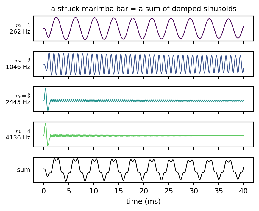
Any linear resonator (FD, FEM): \[ \mathbf{M}\mathbf{u}''=-\mathbf{K}\mathbf{u}-\mathbf{C}\mathbf{u}'+J_{x_e}F \] Mass normalized modes \(\boldsymbol\phi_m\), \(\ \mathbf{u}=\sum_m\boldsymbol\phi_mq_m\): \[ \begin{aligned} q_m''+2\sigma_mq_m'+\omega_m^2q_m&=\phi_m(x_e)\,F\\ y&=\textstyle\sum_m\phi_m(x_o)\,q_m' \end{aligned} \] \(M\) independent oscillators on the exact recursion:

qb = md.a1 * md.q - md.a2 * md.qp    # no force
qn = qb + md.g * phi_e * F           # input weights
y[n] = phi_o @ (qn - md.q) / k       # output weights
Show code
md, pe, po = bar_instrument(261.6, ratio=4)
r = strike(md, pe, po, MH=0.03, KH=1e10, vH=1.5, dur=0.6)
y_parts = []
for m in range(4):                                     # the same strike, one mode at a time (linear: superpose)
    w = np.zeros_like(po); w[m] = po[m]
    y_parts.append(run_modes(md, w, lambda n: pe * (r["F"][n] if n < len(r["F"]) else 0.0), 0.04))
t = 1e3 * np.arange(len(y_parts[0])) * k
fig, axs = plt.subplots(5, 1, figsize=(4.6, 3.8), sharex=True)
for m, (ax, yp) in enumerate(zip(axs, y_parts)):
    ax.plot(t, yp, color=plt.cm.viridis(m / 4), lw=0.9); ax.set_yticks([])
    ax.set_ylabel(f"$m={m + 1}$\n{md.f[m]:.0f} Hz", fontsize=7.5, rotation=0, ha="right", va="center")
axs[4].plot(t, r["y"][:len(t)], color="k", lw=0.9); axs[4].set_yticks([])
axs[4].set_ylabel("sum", fontsize=8, rotation=0, ha="right", va="center")
axs[0].set_title("a struck marimba bar = a sum of damped sinusoids", fontsize=9)
axs[4].set_xlabel("time (ms)")
plt.tight_layout()
plt.show()

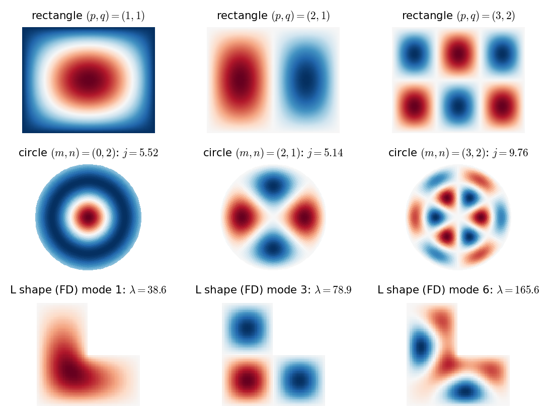
Where the Modes Come From

Analytic (simple shapes)

  • rectangle: \(\sin\cdot\sin\)
  • circle: \(J_m(j_{mn}r/R)\cos m\theta\)
  • free bar: \(\cos\), \(\cosh\)

Numerical (any shape)

  • FD matrix eigenvectors (L shape)
  • FEM (class 16)
  • measured (impact hammer)

Numerical modes inherit dispersion

5 point grid on a square: mode 30 is 6 cents flat.

Show code
fig, axs = plt.subplots(3, 3, figsize=(6.0, 4.4))
xx, yy = np.meshgrid(np.linspace(0, 1, 120), np.linspace(0, 0.8, 96))
for ax, (p, q) in zip(axs[0], [(1, 1), (2, 1), (3, 2)]):
    ax.imshow(np.sin(p * np.pi * xx) * np.sin(q * np.pi * yy / 0.8), cmap="RdBu_r", origin="lower", extent=[0, 1, 0, 0.8])
    ax.set_title(f"rectangle $(p,q)=({p},{q})$", fontsize=8)
rr, tt = np.meshgrid(np.linspace(0, 1, 80), np.linspace(0, 2 * np.pi, 160))
for ax, (m, n) in zip(axs[1], [(0, 2), (2, 1), (3, 2)]):
    z = jn_zeros(m, n)[-1]
    ax.pcolormesh(rr * np.cos(tt), rr * np.sin(tt), jv(m, z * rr) * np.cos(m * tt), cmap="RdBu_r", shading="auto", rasterized=True)
    ax.set_aspect("equal"); ax.set_title(f"circle $(m,n)=({m},{n})$: $j={z:.2f}$", fontsize=8)
for ax, i in zip(axs[2], [0, 2, 5]):
    Z = np.full(XL.shape, np.nan); Z[inL] = VL[:, i]; v = np.nanmax(np.abs(Z))
    ax.imshow(Z, cmap="RdBu_r", vmin=-v, vmax=v, origin="lower", extent=[0, 1, 0, 1])
    ax.set_title(f"L shape (FD) mode {i + 1}: $\\lambda={lamL[i]:.1f}$", fontsize=8)
for ax in axs.flat:
    ax.set_xticks([]); ax.set_yticks([]); [s.set_visible(False) for s in ax.spines.values()]
plt.tight_layout()
plt.show()

Input and Output Weights

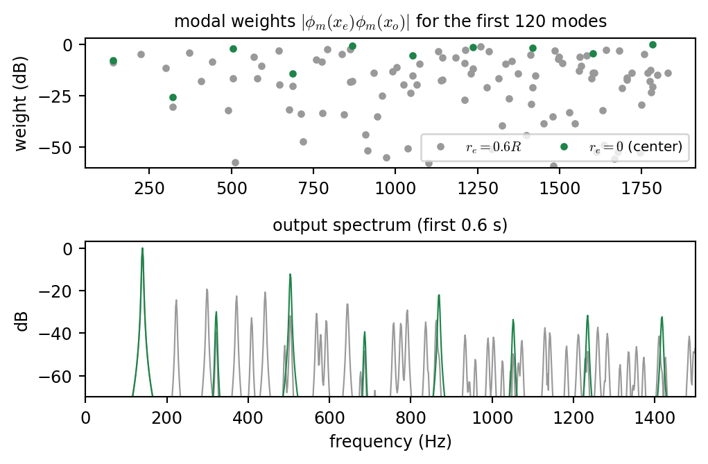
\[ y=\sum_m\underbrace{\phi_m(x_o)\,\phi_m(x_e)}_{\text{weight}}\,(h_m*F) \]

  • Nodal line: that mode is gone
  • Center: only \(m=0\) rings (thud)
  • Off center: every family (tone)
  • Reciprocity: swap \(x_e\), \(x_o\)

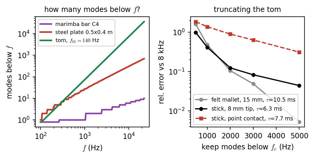
Tom: \(R=15\) cm, \(f_{01}=140\) Hz, 914 modes below 5 kHz.

Show code
fig, axs = plt.subplots(2, 1, figsize=(5.4, 3.6), height_ratios=[1, 1.2])
for tag, col, lab in [("off", "0.6", "$r_e=0.6R$"), ("center", COL["membrane"], "$r_e=0$ (center)")]:
    r, pe, po = tom_runs[tag]
    w = np.abs(pe * po); w = 20 * np.log10(w / w.max() + 1e-6)
    axs[0].plot(TOM["f"][:120], w[:120], "o", color=col, ms=3, label=lab)
    y = r["y"]; Y = np.abs(np.fft.rfft(y[:int(0.6 * fs)] * np.hanning(int(0.6 * fs)))); f = np.fft.rfftfreq(int(0.6 * fs), k)
    axs[1].plot(f, 20 * np.log10(Y / Y.max() + 1e-9), color=col, lw=0.8, label=lab)
axs[0].set_ylim(-60, 3); axs[0].set_ylabel("weight (dB)"); axs[0].legend(fontsize=7.5, ncol=2, loc="lower right")
axs[0].set_title("modal weights $|\\phi_m(x_e)\\phi_m(x_o)|$ for the first 120 modes", fontsize=9)
axs[1].set_xlim(0, 1500); axs[1].set_ylim(-70, 3); axs[1].set_xlabel("frequency (Hz)"); axs[1].set_ylabel("dB")
axs[1].set_title("output spectrum (first 0.6 s)", fontsize=9)
plt.tight_layout()
plt.show()

center strike

off center, \(0.6R\)

Truncation and Damping

Keep modes with

  1. \(f_m<f_s/2\) (no aliasing)
  2. \(f_m\lesssim1/\tau\) (what the contact excites)

Contact size: a point force on a membrane never converges (red); a tip of radius \(a\) does: \[ \phi_m(x_e)\times\frac{2J_1(\beta_ma)}{\beta_ma} \]

Damping: any \(\sigma_m\) per mode, even measured (class 15).

Show code
fig, axs = plt.subplots(1, 2, figsize=(5.6, 2.9))
ff = np.logspace(2, np.log10(fs / 2), 200)
bar_f = BAR[4][0] / BAR[4][0][0] * 261.6
nb = [np.sum(bar_f < f) for f in ff]
pl_ = Plate(fmax=fs / 2); npl = [np.sum(pl_.f < f) for f in ff]
nm = (J01 * ff / 140.0)**2 / 4                                      # j_mn < x: about x^2 / 4 (cos family)
for n_, col, lab in [(nb, COL["bar"], "marimba bar C4"), (npl, COL["plate"], "steel plate 0.5x0.4 m"),
                     (nm, COL["membrane"], "tom, $f_{01}=140$ Hz")]:
    axs[0].loglog(ff, np.maximum(n_, 0.8), color=col, lw=2, label=lab)
axs[0].set_xlabel("$f$ (Hz)"); axs[0].set_ylabel("modes below $f$"); axs[0].legend(fontsize=6.8)
axs[0].set_title("how many modes below $f$?", fontsize=9)
for (name, (e, tc)), col, ls in zip(trunc.items(), ["0.55", "k", COL["plate"]], ["o-", "o-", "s--"]):
    axs[1].semilogy([500, 1000, 2000, 3000, 5000], e, ls, color=col, ms=4, label=f"{name}, $\\tau$={1e3 * tc:.1f} ms")
axs[1].set_xlabel("keep modes below $f_c$ (Hz)"); axs[1].set_ylabel("rel. error vs 8 kHz")
axs[1].legend(fontsize=7); axs[1].set_title("truncating the tom", fontsize=9)
plt.tight_layout()
plt.show()

\(f_c=1\) kHz

\(f_c=3\) kHz

reference, 8 kHz

Cost: Modal vs Finite Differences

finite differences at the CFL limit modal, all modes below Nyquist modal, truncated
tom (\(R=15\) cm, \(f_{01}=140\) Hz) 22,832 points \(\times\) 6 35,864 modes \(\times\) 3 914 modes (5 kHz) \(\times\) 3
steel plate \(0.5\times0.4\) m, 2 mm 720 points \(\times\) 14 691 modes \(\times\) 3 same, exact \(\omega_m\)
precompute none eigenproblem (or formulas) eigenproblem + storage
per sample, this Python bank 0.05 s per s of audio (914 modes)

Modal wins

  • linear resonator, modes known
  • truncate to what is excited
  • exact pitch, any damping, always stable

Modal loses

  • complex shape: big eigenproblem, storage
  • the whole field is needed
  • nonlinear: modes stop being independent

Exciter Coupling

Mallet Meets Modes: One Scalar per Step

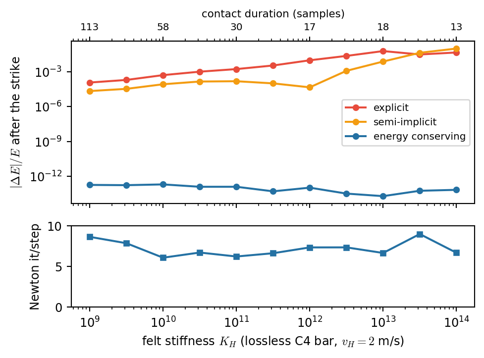
Felt compression \(\eta=u_H-\boldsymbol\phi_e\cdot\mathbf{q}\) (class 13): \[ F=K_H[\eta]_+^{\alpha}=V'(\eta),\qquad M_Hu_H''=-F \] Free update, then add \(F\) to both sides: \[ \eta^{n+1}=\bar\eta-m\,F \] One scalar equation, however many modes.

scheme \(F\) solve
explicit \(V'(\eta^n)\) none
semi-implicit \(K_H[\eta^n]_+^{\alpha-1}\mu_{t\cdot}\eta\) closed form
energy conserving \(\dfrac{V(\eta^{n+1})-V(\eta^{n-1})}{\eta^{n+1}-\eta^{n-1}}\) Newton
m = k**2 / MH + (md.g * pe) @ pe
qb, uHb = md.free(), 2 * uH - uHp
etab = uHb - pe @ qb                    # eta^{n+1} if F = 0
etam = uHp - pe @ md.qp                 # eta^{n-1}
# energy conserving: r = eta^{n+1} - eta^{n-1} solves
#   r + m (V(etam + r) - V(etam)) / r = etab - etam
r = etab - etam
for it in range(50):                    # Newton, class 5
    p, dp = secant_slope(etam, r)       # (V(etam+r)-V(etam))/r, d/dr
    dr = (r + m * p - (etab - etam)) / (1 + m * dp)
    r -= dr
    if abs(dr) < 1e-13 * abs(r): break
F = (etab - etam - r) / m
qn = qb + md.g * pe * F                 # same F, opposite signs
uHn = uHb - k**2 / MH * F

\(V\) convex: one root, and the total energy is conserved exactly.

Explicit, Semi-Implicit, or Energy Conserving?

Show code
fig, axs = plt.subplots(2, 1, figsize=(5.2, 3.9), sharex=True, height_ratios=[2, 1])
for s, col, lab in [("explicit", "#e74c3c", "explicit"), ("semi", "#f39c12", "semi-implicit"), ("ec", COL["modal"], "energy conserving")]:
    axs[0].loglog(KHs, np.maximum(cmp_[s], 1e-16), "o-", color=col, ms=4, label=lab)
axs[0].set_ylabel("$|\\Delta E|/E$ after the strike"); axs[0].legend(fontsize=7.5)
ax2 = axs[0].secondary_xaxis("top"); ax2.set_xticks(KHs[::2]); ax2.set_xticklabels([str(n) for n in nsteps[::2]], fontsize=7.5)
ax2.set_xlabel("contact duration (samples)", fontsize=8)
axs[1].semilogx(KHs, iters, "s-", color=COL["modal"], ms=4)
axs[1].set_ylabel("Newton it/step"); axs[1].set_xlabel("felt stiffness $K_H$ (lossless C4 bar, $v_H=2$ m/s)")
axs[1].set_ylim(0, 10)
plt.tight_layout()
plt.show()

  • Soft (100+ samples): all fine
  • Hard (a few samples): explicit errs up to 6%, semi-implicit 10%
  • Energy conserving: exact, a few Newton steps, only during contact

Rule of thumb

Explicit for felt; energy conserving for sticks and metal beaters.

Hardness, Mass, Velocity

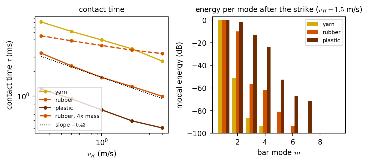
Contact time: \[ \tau\propto\Bigl(\frac{M_H}{K_H}\Bigr)^{\frac1{\alpha+1}}v_H^{\frac{1-\alpha}{1+\alpha}} \]

  • Harder: shorter, brighter
  • Heavier: longer, darker
  • Faster: shorter, brighter
  • Linear felt (\(\alpha=1\)): \(\tau\) ignores \(v_H\)

Modes above \(1/\tau\) stay quiet.

Show code
fig, axs = plt.subplots(1, 2, figsize=(6.2, 3.0))
cols = {"yarn": "#d4ac0d", "rubber": COL["exciter"], "plastic": "#6e2c00", "rubber, 4x mass": COL["exciter"]}
for name, tcs in tc_runs.items():
    axs[0].loglog(vs, 1e3 * tcs, "o-" if "mass" not in name else "o--", color=cols[name], ms=3.5, label=name)
axs[0].loglog(vs, 1e3 * tc_runs["rubber"][2] * vs**(-1.5 / 3.5), "k:", lw=1, label="slope $-0.43$")
axs[0].set_xlabel("$v_H$ (m/s)"); axs[0].set_ylabel("contact time $\\tau$ (ms)"); axs[0].legend(fontsize=6.8)
axs[0].set_title("contact time", fontsize=9)
for i, (name, Em) in enumerate(Em_runs.items()):
    axs[1].bar(np.arange(1, len(Em) + 1) + (i - 1) * 0.27, 10 * np.log10(Em / Em.max() + 1e-12) + 100, width=0.27,
               bottom=-100, color=cols[name], label=name)
axs[1].set_ylim(-100, 3); axs[1].set_xlabel("bar mode $m$"); axs[1].set_ylabel("modal energy (dB)")
axs[1].set_title("energy per mode after the strike ($v_H=1.5$ m/s)", fontsize=9); axs[1].legend(fontsize=6.8)
plt.tight_layout()
plt.show()

yarn
rubber
hard plastic
rubber, 6 m/s

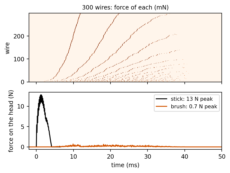
A Brush: Light Bending Wires

Show code: the wire model
def bristle_forces(dur, center, nb=300, a=0.03, dmax=5e-3, T=0.04, t0=0.05, spread=4e-3,
                   d=2e-4, L=0.06, E=2e11, rho=7850.0, Kc=2e3, zeta=0.03, sub=4, seed=3):
    """every wire: tip mass m_b on its bending spring k_b = 3 E I / L^3, the handle pressed by dmax sin(pi t / T);
    the tip touches the head through a linear contact K_c. Returns the force of every wire on the head."""
    rg = np.random.default_rng(seed)
    kb = 3 * E * (np.pi * d**4 / 64) / L**3; mb = 0.24 * rho * np.pi * d**2 / 4 * L; cb = 2 * zeta * np.sqrt(kb * mb)
    rest = rg.random(nb) * spread                                  # the fan: tips at different heights
    r_, th = a * np.sqrt(rg.random(nb)), 2 * np.pi * rg.random(nb)  # tips spread over a disk of radius a
    x, v, h = rest.copy(), np.zeros(nb), k / sub
    F = np.zeros((int(dur * fs), nb))
    for n in range(len(F)):
        dd = dmax * np.sin(np.pi * (n * k - t0) / T) if t0 < n * k < t0 + T else 0.0
        for _ in range(sub):                                        # symplectic Euler, 4 substeps
            fc = Kc * np.maximum(-x, 0.0)
            v += h * (-kb * (x - rest + dd) - cb * v + fc) / mb; x += h * v
            F[n] += fc / sub
    return F, center[0] + r_ * np.cos(th), center[1] + r_ * np.sin(th), dict(kb=kb, mb=mb)

def brush_tap(Mm, md, po, dur, center, **kw):
    """one way: the wires barely see the head move; modal forcing f_m = sum_b phi_m(x_b) F_b(t)"""
    F, X, Y, info = bristle_forces(min(dur, 0.15), center, **kw)
    Fm = F @ mshape(Mm, np.hypot(X, Y), np.arctan2(Y, X))
    return run_modes(md, po, lambda n: Fm[n] if n < len(Fm) else 0.0, dur), F, info

Each wire is a light cantilever (first mode): \[ k_b=\frac{3EI}{L^3} \] \(k_b\approx\) 0.22 N/m, tip mass \(m_b\approx\) 4 mg. Press the handle: tips land one by one, bend, and push the head with \[ F_b=K_c[-x_b]_+ \] Modal forcing: \[ f_m(t)=\sum_b\phi_m(x_b)\,F_b(t) \] The head barely moves the wires: one way coupling, no solve.

Show code
fig, axs = plt.subplots(2, 1, figsize=(5.0, 3.8), sharex=True, height_ratios=[1.2, 1])
t_ms = 1e3 * (np.arange(len(F_tap)) * k - 0.05)
o = np.argsort(np.argmax(F_tap > 0, axis=0))
axs[0].pcolormesh(t_ms, np.arange(F_tap.shape[1]), 1e3 * F_tap[:, o].T, cmap="Oranges", shading="auto", rasterized=True, vmax=8)
axs[0].set_ylabel("wire"); axs[0].set_title(f"{F_tap.shape[1]} wires: force of each (mN)", fontsize=9)
Fs_ = r_stick["F"]
axs[1].plot(1e3 * np.arange(len(Fs_)) * k, Fs_, color="k", lw=1.4, label=f"stick: {Fs_.max():.0f} N peak")
axs[1].plot(t_ms, F_tap.sum(1), color=COL["exciter"], lw=1.4, label=f"brush: {F_tap.sum(1).max():.1f} N peak")
axs[1].set_xlim(-2, 50); axs[1].set_xlabel("time (ms)"); axs[1].set_ylabel("force on the head (N)"); axs[1].legend(fontsize=8)
plt.tight_layout()
plt.show()

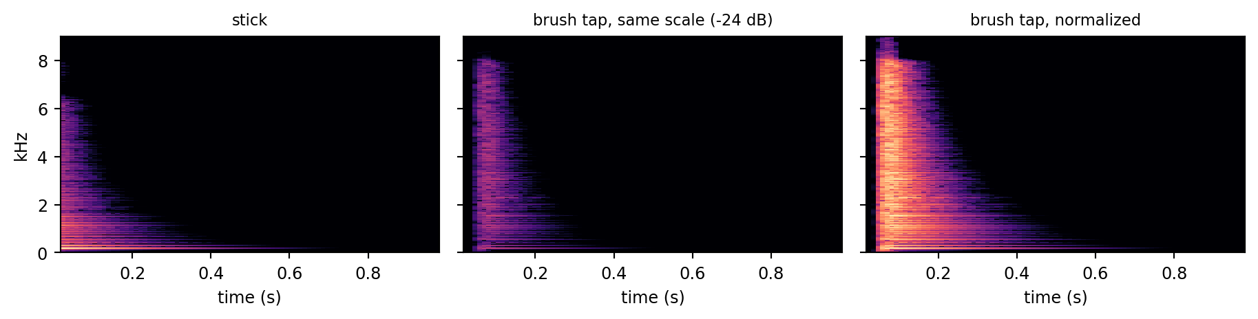
Stick vs Brush

Show code
smax = lambda y, win=2048: max(np.abs(np.fft.rfft(y[i:i + win] * np.hanning(win))).max() for i in range(0, len(y) - win, win // 4))
fig, axs = plt.subplots(1, 3, figsize=(9.6, 2.5), sharey=True)
ref = smax(r_stick["y"])
for ax, (y, title, nrm) in zip(axs, [(r_stick["y"], "stick", ref), (y_tap, f"brush tap, same scale ({tap_db:.0f} dB)", ref),
                                     (y_tap, "brush tap, normalized", None)]):
    show_spec(ax, y, title, fmax=9, vmin=-80, norm=nrm)
    ax.set_xlabel("time (s)")
axs[0].set_ylabel("kHz")
plt.tight_layout()
plt.show()

stick

brush tap, same gain

brush tap, normalized

A Friction Drum: Rubbing a Stick

Show code: the friction drum
CUICA = membrane_modes(R=0.1, f01=500.0, fmax=12000.0, rho_s=0.3)
CU0 = {key: (v[CUICA["m"] == 0] if isinstance(v, np.ndarray) else v) for key, v in CUICA.items()}   # center drive: m = 0

def friction_drum(vB, FB, tune, dur, ms=0.002, a=0.006, T60=0.5, push=lambda t: 0.0):
    """stick of mass ms glued at the center, rubbed at vB(t) with grip FB(t); tune(t) scales every frequency (thumb)"""
    w, po = mshape(CU0, 0.0)[0] * patch(CU0, a), mshape(CU0, 0.3 * CU0["R"])[0]
    sig = 3 * np.log(10) * (1 + CU0["f"] / 1500) / T60
    d = 1 + sig * k; a2, g = (1 - sig * k) / d, k**2 / d
    c2 = (g * w * w).sum(); den = 1 + ms * c2 / k**2                # head displacement per newton; stick inertia
    q, qp, v = np.zeros(len(w)), np.zeros(len(w)), 0.0
    y, vr, its = np.zeros(int(dur * fs)), np.zeros(int(dur * fs)), []
    for n in range(len(y)):
        t = n * k
        qb = 2 * np.cos(2 * np.pi * CU0["f"] * tune(t) * k) / d * q - a2 * qp     # exact recursion, retuned
        ub, u, um = w @ qb, w @ q, w @ qp
        G0 = push(t) - ms * (ub - 2 * u + um) / k**2
        v0 = (ub + c2 * G0 / den - um) / (2 * k) - vB(t)
        v, it = fric_solve(v0, c2 / (2 * k * den) * FB(t), v)          # v - v0 + c F_B phi(v) = 0
        qn = qb + g * w * (G0 - FB(t) * phi_f(v)) / den                 # force on the head
        y[n], vr[n] = po @ (qn - q) / k, v; its.append(it)
        qp, q = q, qn
    return y, vr, np.array(its), c2 / (2 * k * den)

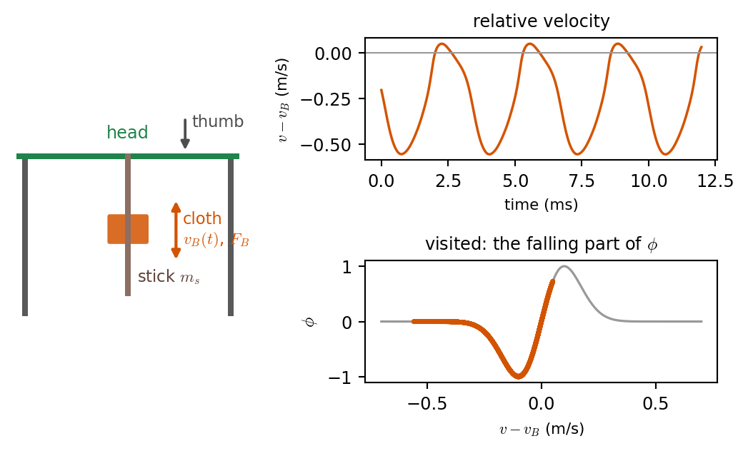
Friction on the stick (class 16 bow): \[ F=-F_B\,\phi(v-v_B) \] The stick (mass \(m_s\)) moves with the head center: only the \(m=0\) modes, 18 of them.

One scalar per step, as for the bow: \[ v-v_0+c\,F_B\,\phi(v)=0 \] \(cF_B\max(-\phi')=\) 0.03 \(<1\): one root, 3.0 Newton steps.

Falling \(\phi\) feeds energy: a self-sustained oscillation.

Thumb: every \(\omega_m\to s(t)\,\omega_m\).

Show code
fig = plt.figure(figsize=(5.4, 3.4)); gs = fig.add_gridspec(2, 2, width_ratios=[1, 1.4])
ax = fig.add_subplot(gs[:, 0])                                      # sketch of a cuica, in cm
ax.plot([-9, -9], [0, 14], color="0.35", lw=3); ax.plot([9, 9], [0, 14], color="0.35", lw=3)
ax.plot([-9.5, 9.5], [14, 14], color=COL["membrane"], lw=3); ax.text(0, 15.6, "head", ha="center", color=COL["membrane"], fontsize=9)
ax.plot([0, 0], [14, 2], color="#8d6e63", lw=3); ax.text(0.8, 3, "stick $m_s$", fontsize=8.5, color="#5d4037")
ax.add_patch(plt.matplotlib.patches.FancyBboxPatch((-1.6, 6.5), 3.2, 2.2, boxstyle="round,pad=0.2", fc=COL["exciter"], ec="none", alpha=0.85))
ax.annotate("", xy=(4.2, 4.6), xytext=(4.2, 10.4), arrowprops=dict(arrowstyle="<|-|>", color=COL["exciter"], lw=1.6))
ax.text(4.8, 7.5, "cloth\n$v_B(t)$, $F_B$", fontsize=8.5, color=COL["exciter"], va="center")
ax.annotate("", xy=(5, 14.2), xytext=(5, 17.5), arrowprops=dict(arrowstyle="-|>", color="0.3", lw=1.4))
ax.text(5.6, 16.6, "thumb", fontsize=8.5, color="0.3")
ax.set_xlim(-10, 12); ax.set_ylim(0, 18.5); ax.set_aspect("equal"); ax.axis("off")
n0 = int(0.2 * fs); seg = vr_rub[n0:n0 + int(0.012 * fs)]
a1_, a2_ = fig.add_subplot(gs[0, 1]), fig.add_subplot(gs[1, 1])
a1_.plot(1e3 * np.arange(len(seg)) * k, seg, color=COL["exciter"], lw=1.3); a1_.axhline(0, color="0.6", lw=0.8)
a1_.set_xlabel("time (ms)", fontsize=8); a1_.set_ylabel("$v-v_B$ (m/s)", fontsize=8); a1_.set_title("relative velocity", fontsize=9)
vv = np.linspace(-0.7, 0.7, 400)
a2_.plot(vv, phi_f(vv), color="0.6", lw=1.2); a2_.plot(seg, phi_f(seg), color=COL["exciter"], lw=2.5)
a2_.set_xlabel("$v-v_B$ (m/s)", fontsize=8); a2_.set_ylabel("$\\phi$", fontsize=9)
a2_.set_title("visited: the falling part of $\\phi$", fontsize=9)
plt.tight_layout()
plt.show()
Hear the Friction Drum

Show code
fig, axs = plt.subplots(1, 2, figsize=(9.6, 2.7), width_ratios=[1.6, 1])
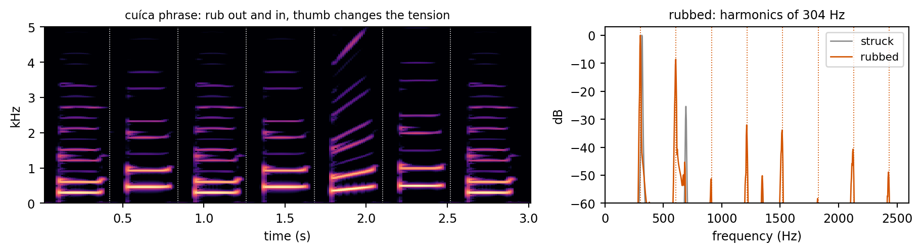
show_spec(axs[0], y_cuica, "cuíca phrase: rub out and in, thumb changes the tension", fmax=5, vmin=-70)
for i in range(1, len(TUNE)):
    axs[0].axvline(i * Ts, color="w", lw=0.6, ls=":")
axs[0].set_xlabel("time (s)"); axs[0].set_ylabel("kHz")
for y, col, lab in [(y_hit, "0.55", "struck"), (y_rub, COL["exciter"], "rubbed")]:
    seg = y[int(0.1 * fs):int(0.4 * fs)]; Y = np.abs(np.fft.rfft(seg * np.hanning(len(seg)))); f = np.fft.rfftfreq(len(seg), k)
    axs[1].plot(f, 20 * np.log10(Y / Y.max() + 1e-9), color=col, lw=1, label=lab)
f_rub = period_f0(y_rub[int(0.15 * fs):int(0.3 * fs)])
for h_ in range(1, 9):
    axs[1].axvline(h_ * f_rub, color=COL["exciter"], ls=":", lw=0.7)
axs[1].set_xlim(0, 2600); axs[1].set_ylim(-60, 3); axs[1].set_xlabel("frequency (Hz)"); axs[1].set_ylabel("dB")
axs[1].set_title(f"rubbed: harmonics of {f_rub:.0f} Hz", fontsize=9); axs[1].legend(fontsize=8)
plt.tight_layout()
plt.show()
struck once (inharmonic)

rubbed (pitched)

rubbed + thumb (cuíca)

Instruments

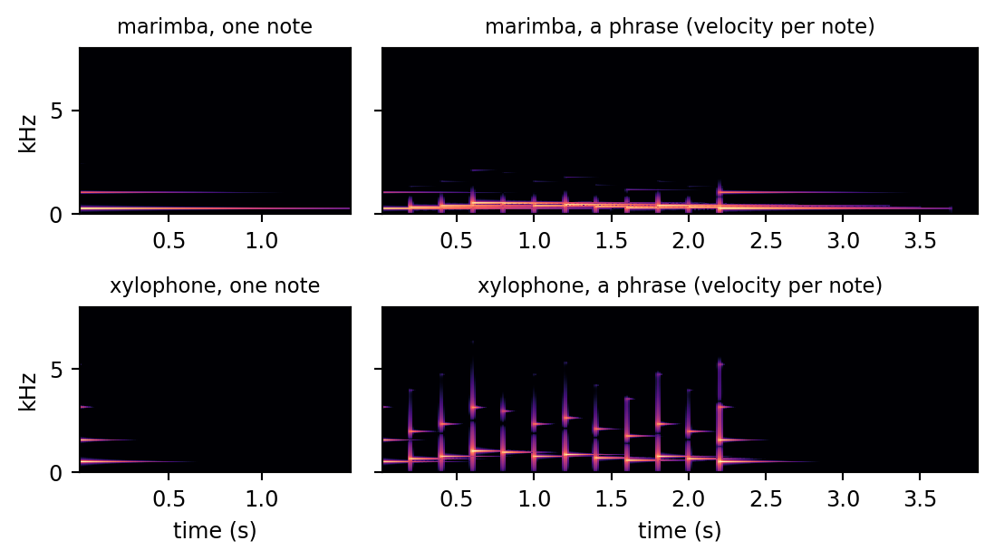
Marimba and Xylophone

Carved bar modes (class 15), scaled to each note:

marimba xylophone
\(f_2/f_1\) \(4\) (2 octaves) \(3\) (octave + 5th)
mallet yarn, \(K_H=3\times10^9\) plastic, \(K_H=3\times10^{11}\)
ring, \(T_{60}\) at C4 2 s 0.7 s
sounds as written an octave up

A phrase: one bank + mallet per note, summed.

Not modeled: the resonator tubes (next class).

Show code
fig, axs = plt.subplots(2, 2, figsize=(5.8, 3.3), width_ratios=[1, 2.2], sharey="row")
for row, (y1, yP, nm) in enumerate([(y_mar1, y_marP, "marimba"), (y_xyl1, y_xylP, "xylophone")]):
    show_spec(axs[row, 0], y1, f"{nm}, one note", fmax=8, vmin=-75)
    show_spec(axs[row, 1], yP, f"{nm}, a phrase (velocity per note)", fmax=8, vmin=-75)
    axs[row, 0].set_ylabel("kHz")
for ax in axs[1]:
    ax.set_xlabel("time (s)")
plt.tight_layout()
plt.show()
marimba C4
xylophone C5
marimba phrase
xylophone phrase

Drums: The Bessel Series

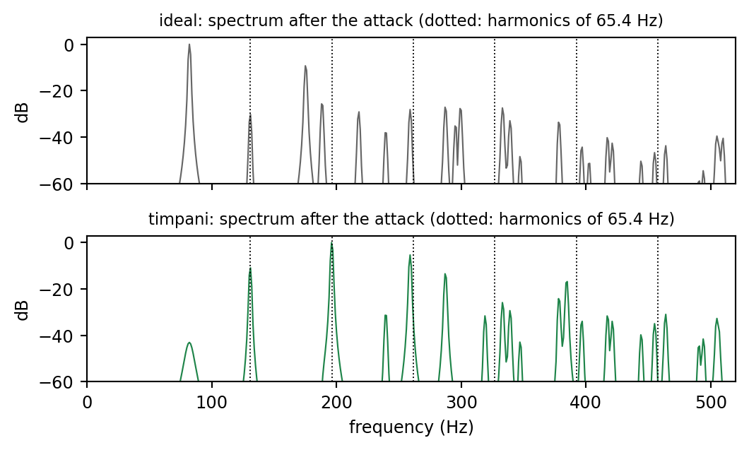
Ideal membrane, \(f_{mn}\propto j_{mn}\): \[ 1:1.59:2.14:2.30:2.65 \] Inharmonic: a vague pitch.

Timpani: air loading lowers the low modes; the \((m,1)\) modes land near \[ 1:1.5:2:2.5:3 \] harmonics 2 to 6 of a missing fundamental.

Here: edit the modes (measured ratios, short \(T_{60}\) for \((0,n)\)).

Show code
fig, axs = plt.subplots(2, 1, figsize=(5.6, 3.4), sharex=True)
for ax, (name, y), col in zip(axs, timp.items(), ["0.4", COL["membrane"]]):
    n = int(1.0 * fs); Y = np.abs(np.fft.rfft(y[int(0.05 * fs):int(0.05 * fs) + n] * np.hanning(n))); f = np.fft.rfftfreq(n, k)
    ax.plot(f, 20 * np.log10(Y / Y.max() + 1e-9), color=col, lw=0.8)
    for h_ in range(2, 8):
        ax.axvline(65.4 * h_, color="k", ls=":", lw=0.7)
    ax.set_ylim(-60, 3); ax.set_ylabel("dB"); ax.set_title(f"{name}: spectrum after the attack (dotted: harmonics of 65.4 Hz)", fontsize=8.5)
axs[1].set_xlim(0, 520); axs[1].set_xlabel("frequency (Hz)")
plt.tight_layout()
plt.show()
ideal membrane (\(R=33\) cm)

modes retuned as a timpani

A Struck Plate: Louder Is Only Louder

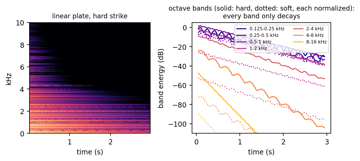
Steel plate, \(H=2\) mm, 691 modes, 100 g mallet.

Linear modes never exchange energy: \[ \mathfrak h_m(t)=\mathfrak h_m(0^+)\,e^{-2\sigma_mt} \] The spectrum is set during the contact, then only decays: louder is only louder.

A real gong struck hard brightens after the strike. Impossible here.

Show code
edges = [125, 250, 500, 1000, 2000, 4000, 8000, 16000]
fig, axs = plt.subplots(1, 2, figsize=(6.2, 3.0), width_ratios=[1, 1.15])
show_spec(axs[0], lin_pl["hard"]["y"], "linear plate, hard strike", fmax=10, vmin=-80)
axs[0].set_xlabel("time (s)"); axs[0].set_ylabel("kHz")
for tag, ls in [("soft", ":"), ("hard", "-")]:
    tb, Eb = band_energy(lin_pl[tag]["y"], edges)
    for i in range(len(edges) - 1):
        axs[1].plot(tb, Eb[:, i] - Eb[:, 0].max(), ls, color=plt.cm.plasma(i / 7), lw=1.3,
                    label=f"{edges[i] / 1e3:g}-{edges[i + 1] / 1e3:g} kHz" if tag == "hard" else None)
axs[1].set_ylim(-110, 5); axs[1].set_xlabel("time (s)"); axs[1].set_ylabel("band energy (dB)")
axs[1].set_title("octave bands (solid: hard, dotted: soft, each normalized):\nevery band only decays", fontsize=8.5)
axs[1].legend(fontsize=6, ncol=2, loc="upper right")
plt.tight_layout()
plt.show()
linear, soft strike (0.3 m/s)

linear, hard strike (6 m/s)

Try It: Percussion Lab

Nonlinear Modal Synthesis

Berger Plate: One Global Tension

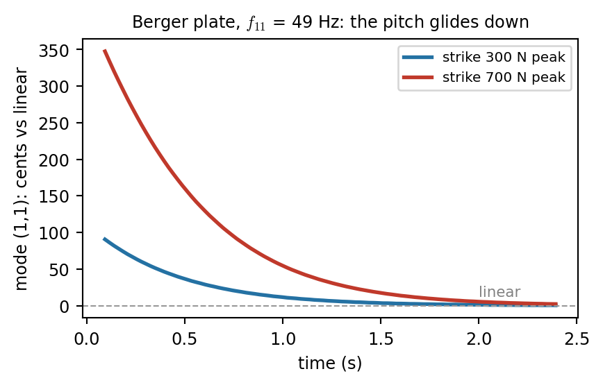
Stretching adds one global tension (Kirchhoff-Carrier in 2D): \[ \rho Hu_{tt}=-D\nabla^4u+T(u)\,\nabla^2u \] \[ T(u)=\frac{6D}{|\Omega|H^2}\int_{\Omega}|\nabla u|^2dA \] Modal form: every mode sees one scalar \[ q_s''+\omega_s^2q_s=-w\,g\,\beta_s^2q_s,\quad g=\sum_p\beta_p^2q_p^2 \] Conservative: \(g\) averaged over two steps, a rank one solve per step.

Pitch glides down (opera gong), but no crash.

Show code
HB, wB = np.diag(P5.b2)[None], [6 * P5.kappa**2 / (P5.Lx * P5.Ly * P5.H**2)]   # H_1 = diag(beta^2)
fig, ax = plt.subplots(figsize=(4.6, 3.0))
t_, ref = pitch_track(berger_lin, P5.f[0], lo=0.9, hi=1.4)
for (F, y), col in zip(berger.items(), [COL["modal"], COL["plate"]]):
    t_, fr = pitch_track(y, P5.f[0], lo=0.9, hi=1.4)
    ax.plot(t_, 1200 * np.log2(fr / ref), color=col, lw=2, label=f"strike {F:.0f} N peak")
ax.axhline(0, color="0.6", ls="--", lw=0.8); ax.text(2.0, 12, "linear", color="0.5", fontsize=8)
ax.set_xlabel("time (s)"); ax.set_ylabel("mode (1,1): cents vs linear")
ax.set_title(f"Berger plate, $f_{{11}}$ = {P5.f[0]:.0f} Hz: the pitch glides down", fontsize=9); ax.legend(fontsize=7.5)
plt.tight_layout()
plt.show()
linear
Berger, 300 N
Berger, 700 N

Von Kármán Plate in Modal Form

Deflection \(u\), Airy stress \(\Phi\): \[ \begin{aligned} \rho H\,u_{tt}&=-D\nabla^4u+\mathrm{L}(\Phi,u)\\ \nabla^4\Phi&=-\tfrac{EH}{2}\,\mathrm{L}(u,u) \end{aligned} \] \(\mathrm{L}(f,g)=f_{xx}g_{yy}+f_{yy}g_{xx}-2f_{xy}g_{xy}\): the stress varies over the plate.

Expand in plate modes \(\phi_p\) and stress modes \(\Psi_n\). One coupling tensor: \[ H^n_{pq}=\int_{\Omega}\Psi_n\,\mathrm{L}(\phi_p,\phi_q)\,dA \]

Modal von Kármán \[ q_s''+2\sigma_sq_s'+\omega_s^2q_s=-\sum_nw_n\,g_n\,(\mathbf H^n\mathbf q)_s+f_s \] \[ g_n=\mathbf q^\top\mathbf H^n\mathbf q,\qquad w_n=\frac{E}{2\rho\,\zeta_n^4} \]

  • Cubic: every mode with every pair
  • Berger: one stress mode, \(\mathbf H^1=\operatorname{diag}(\beta^2)\)
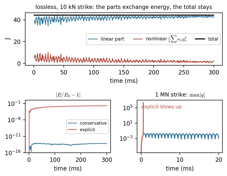
  • Potential \(\frac14\sum_nw_ng_n^2\ge0\)

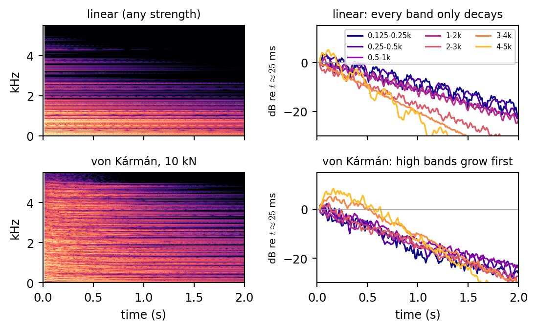
Modes at \(f_a,f_b\) drive \(f_a\pm f_b,\dots\): energy cascades up (the crash).

Building the Coupling Tensor

Sines everywhere: every term of \(\mathrm{L}(\phi_p,\phi_q)\) separates into 1D integrals in \(x\) and \(y\).

sn = lambda n, z: np.sin(np.pi * np.outer(n, z))
cs = lambda n, z: np.cos(np.pi * np.outer(n, z))
X1 = np.einsum("nx,ax,bx->nab", sn(s, xq), sn(p, xq), sn(p, xq)) * Lx / nq
X2 = np.einsum("nx,ax,bx->nab", sn(s, xq), cs(p, xq), cs(p, xq)) * Lx / nq
# ... Y1, Y2 the same in y
H = c * ((np.outer(a**2, b**2) + np.outer(b**2, a**2)) * X1 * Y1
         - 2 * np.outer(a * b, a * b) * X2 * Y2)

Other shapes: the same integrals on an FEM mesh.

linear bank modal von Kármán
state \(2M\) \(2M\)
tensor none \(N_\Psi M^2\)
ops per step \(\approx3M\) \(\approx2N_\Psi M^2+N_\Psi^2M\)
this plate \(M=\) 148 \(N_\Psi=\) 30: 657,120 entries
measured 0.05 ms/step (2.0\(\times\) real time)
precompute 0.8 s
  • Only 25% of \(\mathbf H\) is nonzero
  • A large plate (\(M\approx3\times10^4\)): \(\sim10^{10}\) entries, so couple a subset

A Conservative Scheme

As for the cubic oscillator, use half steps: \[ g_n^{n+\frac12}=\mathbf q^{n+1}\cdot\mathbf H^n\mathbf q^n \] and average \(g_n^{n\pm\frac12}\). The energy is conserved, and the update is linear in \(\mathbf q^{n+1}\): \[ (\mathbf D+\mathbf W\mathbf W^\top)\,\mathbf q^{n+1}=\mathbf r \] diagonal + rank \(N_\Psi\): one small solve (Woodbury), no Newton.

B = (Hm @ q).reshape(NP, -1)        # rows H_n q^n
W = B.T * np.sqrt(0.5 * k**2 * w)
Dr, DW = rhs / d, W / d[:, None]
qn = Dr - DW @ np.linalg.solve(
    np.eye(NP) + W.T @ DW, W.T @ Dr)
Show code
fig, axs = plt.subplots(2, 2, figsize=(5.0, 3.9), height_ratios=[1, 1])
ax = plt.subplot(2, 1, 1); axs[0, 0].remove(); axs[0, 1].remove()
tE = (T_STRIKE + 20 * np.arange(len(E_ec))) * k * 1e3
ax.plot(tE, E_ec[:, 0], color=COL["modal"], lw=1, label="linear part")
ax.plot(tE, E_ec[:, 1], color=COL["plate"], lw=1, label="nonlinear $\\frac{1}{4}\\sum w_n g_n^2$")
ax.plot(tE, E_ec.sum(1), color="k", lw=1.6, label="total")
ax.set_xlabel("time (ms)"); ax.set_ylabel("J"); ax.legend(fontsize=7, ncol=3, loc="center right")
ax.set_title("lossless, 10 kN strike: the parts exchange energy, the total stays", fontsize=8.5)
for E_, col, lab in [(E_ec, COL["modal"], "conservative"), (E_ex, "#e74c3c", "explicit")]:
    tot = E_.sum(1); axs[1, 0].semilogy(tE[:len(tot)], np.abs(tot / tot[0] - 1) + 1e-17, color=col, lw=1, label=lab)
axs[1, 0].set_ylim(1e-16, 1); axs[1, 0].set_xlabel("time (ms)"); axs[1, 0].set_title("$|E/E_0-1|$", fontsize=8.5)
axs[1, 0].legend(fontsize=6.5)
for sch, col in [("ec", COL["modal"]), ("explicit", "#e74c3c")]:
    axs[1, 1].semilogy(1e3 * np.arange(len(blow[sch])) * k, blow[sch], color=col, lw=1.4)
axs[1, 1].set_xlabel("time (ms)"); axs[1, 1].set_title("1 MN strike: $\\max|q|$", fontsize=8.5)
axs[1, 1].text(0.05, 0.85, "explicit blows up", color="#e74c3c", fontsize=7.5, transform=axs[1, 1].transAxes)
plt.tight_layout()
plt.show()
Hear the Cascade

Show code
fig, axs = plt.subplots(2, 2, figsize=(5.8, 3.6), sharex=True)
show_spec(axs[0, 0], cascade_lin, "linear (any strength)", fmax=5.5, vmin=-80)
show_spec(axs[1, 0], cascade[1e4], "von Kármán, 10 kN", fmax=5.5, vmin=-80)
edges = [125, 250, 500, 1000, 2000, 3000, 4000, 5000]
for ax, y, title in [(axs[0, 1], cascade_lin, "linear: every band only decays"), (axs[1, 1], cascade[1e4], "von Kármán: high bands grow first")]:
    tb, Eb = band_energy(y, edges, win=2048, hop=512)
    for i in range(len(edges) - 1):                     # each band relative to its level just after the strike
        ax.plot(tb, Eb[:, i] - Eb[0, i], color=plt.cm.plasma(i / 7), lw=1.2, label=f"{edges[i] / 1e3:g}-{edges[i + 1] / 1e3:g}k")
    ax.axhline(0, color="0.6", lw=0.6); ax.set_ylim(-30, 15); ax.set_title(title, fontsize=8.5); ax.set_xlim(0, 2)
    ax.set_ylabel("dB re $t\\approx25$ ms", fontsize=7.5)
axs[0, 1].legend(fontsize=5.5, ncol=3, loc="upper right")
for ax in axs[:, 0]:
    ax.set_ylabel("kHz")
for ax in axs[1]:
    ax.set_xlabel("time (s)")
plt.tight_layout()
plt.show()
148 coupled modes, same 1 ms force, clips normalized.

linear (identical at every strength) von Kármán, 2 kN: almost linear von Kármán, 10 kN: the shimmer builds up von Kármán, 30 kN: crash

Nonlinear Plate Reverb

From Linear to Nonlinear Plate Reverb

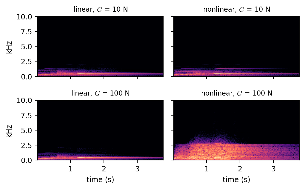
Class 15 plate reverb + von Kármán:

  • 1524 modes, the lowest 250 coupled (to 2.7 kHz)
  • input force \(F(t)=G\,x(t)\)

Nonlinear once the plate moves about its thickness:

\(G\) (peak force) max \(\lvert u\rvert/H\)
10 N 0.06
100 N 1.8

Cost: 1.9 s per second of audio.

Show code
fig, axs = plt.subplots(2, 2, figsize=(5.4, 3.4), sharex=True, sharey=True)
for i, tag in enumerate(["low", "high"]):
    for j, nl_ in enumerate([False, True]):
        show_spec(axs[i, j], reverb[(tag, nl_)][0], f"{'nonlinear' if nl_ else 'linear'}, $G$ = {'10 N' if tag == 'low' else '100 N'}",
                  fmax=10, vmin=-80)
for ax in axs[:, 0]:
    ax.set_ylabel("kHz")
for ax in axs[1]:
    ax.set_xlabel("time (s)")
plt.tight_layout()
plt.show()
Listen: Linear vs Nonlinear Reverb

Input, dry marimba:

small input (\(G=10\) N) large input (\(G=100\) N)
linear plate
nonlinear plate
  • Linear: a filter; both clips sound the same
  • Nonlinear, small: same as linear
  • Nonlinear, large: a sizzling tail with components not in the input

Level dependent effects

Must be nonlinear: no linear filter reacts to how hard it is driven.

Functional Transformation Method

FTM: Transform Space and Time

Stiff lossy string (class 15), simply supported: \[ u_{tt}+2\sigma_0u_t-2\sigma_1u_{txx}-\gamma^2u_{xx}+\kappa^2u_{xxxx}=f(x,t) \]

  1. Laplace in time: \(\partial_t\to s\)
  2. Sturm-Liouville in space, kernel \(K=\sin\beta_\mu x\): \(\ \partial_{xx}\to-\beta_\mu^2\)
  3. Each \(\mu\) is now one algebraic equation: \[ \bar U_\mu(s)=\frac{\bar F_\mu(s)}{s^2+2\sigma_\mu s+\omega_\mu^2+\sigma_\mu^2} \] \[ \sigma_\mu=\sigma_0+\sigma_1\beta_\mu^2,\quad \omega_\mu^2=\gamma^2\beta_\mu^2+\kappa^2\beta_\mu^4-\sigma_\mu^2 \]
  4. Inverse: a series in \(K(\mu,x)\).

Transfer function \(x_e\to x_o\): \[ H(s)=\sum_\mu\frac{K(\mu,x_o)\,K(\mu,x_e)}{N_\mu\,(s-s_\mu)(s-s_\mu^*)} \] Exact poles \(s_\mu=-\sigma_\mu\pm j\omega_\mu\).

Modal synthesis, derived

Frequencies and decays straight from the PDE, no grid.

Impulse Invariance: Each Mode Exactly

Impulse invariance: sample each mode’s impulse response. With \(R_\mu=e^{-\sigma_\mu k}\): \[ H_\mu(z)=\frac{c_\mu\,z^{-1}}{1-2R_\mu\cos(\omega_\mu k)z^{-1}+R_\mu^2z^{-2}} \] Poles \(z_\mu=e^{s_\mu k}\): the class 13 exact recursion.

  • No dispersion: \(\omega_\mu,\sigma_\mu\) exact
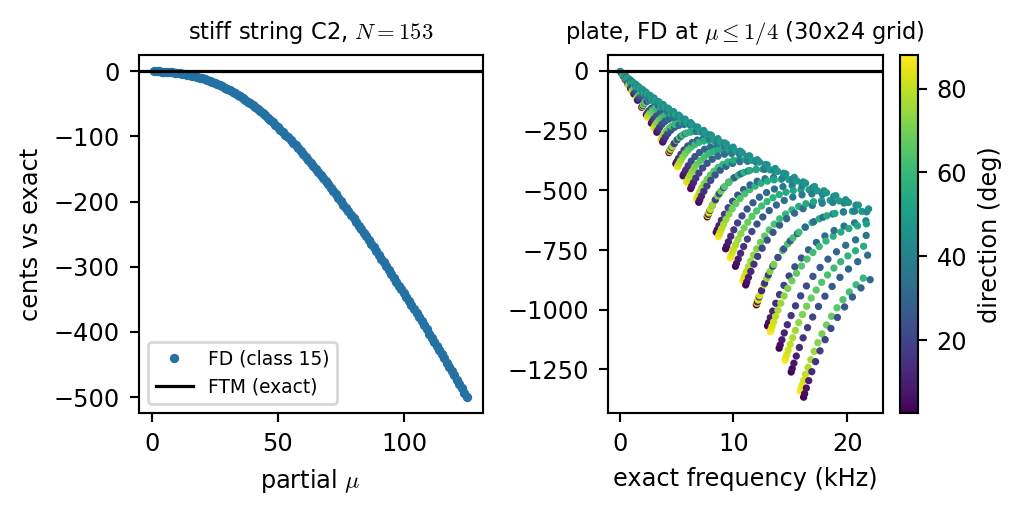
  • FD on a rectangle = a modal bank with wrong frequencies (right)
Show code
fig, axs = plt.subplots(1, 2, figsize=(5.4, 2.8))
axs[0].plot(mu_[okS], 1200 * np.log2(f_fd_s[okS] / f_ftm_s[okS]), "o", color=COL["modal"], ms=2.5, label="FD (class 15)")
axs[0].axhline(0, color="k", lw=1.2, label="FTM (exact)")
axs[0].set_xlabel("partial $\\mu$"); axs[0].set_ylabel("cents vs exact")
axs[0].set_title(f"stiff string C2, $N={Ns}$", fontsize=8.5); axs[0].legend(fontsize=7)
sc = axs[1].scatter(PLf.f[grid] / 1e3, 1200 * np.log2(f_fd_p[grid] / PLf.f[grid]), c=ang[grid], s=3, cmap="viridis")
axs[1].axhline(0, color="k", lw=1.2)
axs[1].set_xlabel("exact frequency (kHz)"); axs[1].set_title(f"plate, FD at $\\mu\\leq1/4$ ({Nx}x{Ny} grid)", fontsize=8.5)
plt.colorbar(sc, ax=axs[1], label="direction (deg)")
plt.tight_layout()
plt.show()
plate, FD frequencies (\(\mu\le\frac14\))

plate, FTM (impulse invariant, exact)

Nonlinear FTM: A Feedback Loop

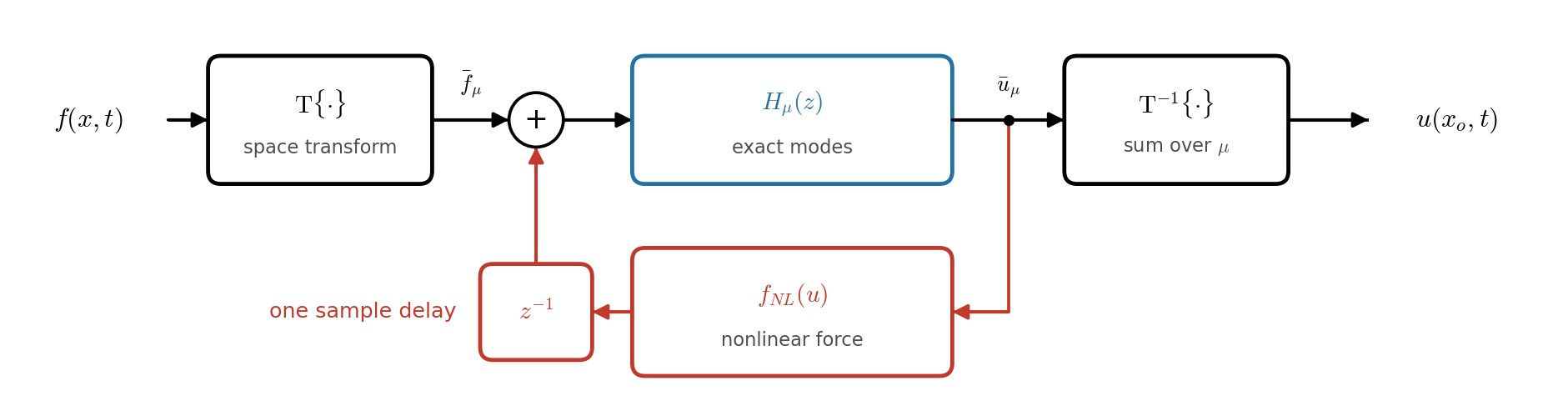
\[ \bar u_\mu^{n+1}=2R_\mu\cos(\omega_\mu k)\,\bar u_\mu^n-R_\mu^2\,\bar u_\mu^{n-1}+c_\mu\bigl(\bar f_\mu^n+\bar f_{NL,\mu}^{\,n}\bigr) \]

  • Nonlinear term moved to the input, fed back one sample later
  • In modal coordinates: today’s explicit scheme
  • Cheap, but no energy guarantee (the 1 MN test)
  • Safer: the half step scheme, one small solve

Choosing a Method

Finite Differences vs Modal vs FTM

finite differences modal (FD, FEM modes) FTM (analytic modes)
frequencies dispersion, tied to \(k\) by CFL mesh error, refine freely exact
damping fixed by the PDE any \(\sigma_m\), even measured from the PDE
stability (linear) CFL always always
cost per sample stencil \(\times\) grid \(3M\), truncate \(3M\), truncate
precompute none eigenproblem, store \(\phi_m\) formulas
shapes any any (FEM) simple shapes only
nonlinearity natural, local tensor \(N_\Psi M^2\) feedback (explicit)
output the whole field points points

Checklist

  1. Linear, simple shape: FTM
  2. Linear, complex shape: FEM modes
  1. Weakly nonlinear, few modes: modal + tensor
  2. Strongly nonlinear, many modes: FD

Looking Ahead

Where These Ideas Come Back

  • Wind Instruments and Digital Waveguides (next class)
    • the reed: a self-sustained oscillator, like the rubbed stick
    • the bore as delay lines (class 14); the marimba’s resonator tubes
  • Sound Effects
    • impacts: mallet + modal bank of everyday objects
    • squeaks, creaks: friction; rattles, scrapes: many light contacts
    • real time through modal truncation
  • Projects: Korean percussion
    • jing, kkwaenggwari: nonlinear gongs
    • buk, janggu: membranes; pyeongyeong: FEM stone modes

Recap

Recap on Today’s ILO

  • Modal synthesis: independent oscillators; truncate, damp, and weight each mode.
  • Exciters: one scalar equation per step
    • mallet: energy conserving (Newton) for hard contacts
    • brush: hundreds of light bending wires, very quiet
    • rubbed stick: friction, a self-sustained, pitched tone
  • Instruments: tuned bars, inharmonic membranes, dense plates.
  • Nonlinear modes: Berger glides, von Kármán crashes; the half step scheme conserves energy.
  • FTM: exact modes from the PDE; impulse invariance = the exact recursion.