Wind Instruments and Digital Waveguides


Topics in Digital Heritage:
Numerical Methods for Digital Reconstruction

Jin Woo Lee

KAIST

Fall 2026

Recap

Last Time: Exciter, Resonator, Shared Force

  • Coupled parts: exciter and resonator share one interface variable, solved by one scalar equation per step (class 16, class 17)
  • Digital waveguide: at \(\lambda=1\) d’Alembert’s two traveling waves move one cell per step, so two delay lines compute the ideal string exactly in \(O(1)\) per sample (class 14)
  • Self-sustained oscillation starts at a Hopf bifurcation (class 13)
  • Newton for one scalar root (class 5)

Today: the air column is (almost) the ideal 1D wave equation, so the waveguide becomes the main tool.

Show code
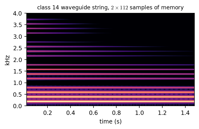
M = int(round(fs / (2 * 196.0)))                       # G3: two delay lines of M samples each
x = np.arange(M) / M; u0 = np.where(x < 0.2, x / 0.2, (1 - x) / 0.8)
r, q = u0 / 2, u0 / 2; out = np.zeros(int(1.5 * fs)); last = 0.0
for n in range(len(out)):
    rr, qq = r[-1], q[0]                               # waves arriving at the two ends
    r = np.r_[-qq, r[:-1]]; refl = -0.998 * 0.5 * (rr + last); last = rr
    q = np.r_[q[1:], refl]                             # reflect with a two-tap average (loop filter)
    out[n] = r[M // 5] + q[M // 5]
save_wav("recap_dwg_string", out)
fig, ax = plt.subplots(figsize=(4.4, 2.9))
show_spec(ax, out, f"class 14 waveguide string, $2\\times{M}$ samples of memory")
ax.set_xlabel("time (s)"); ax.set_ylabel("kHz")
plt.tight_layout()
plt.show()

the class 14 waveguide string

Component Model of a Wind Instrument

instrument exciter bore coupling model today
clarinet single reed (closes with pressure) cylinder two-way reflection table, then a mass-spring reed
saxophone the same reed cone two-way Kelly–Lochbaum cone
trumpet lips (open with pressure) cylinder + bell two-way lip oscillator, bell by scattering
flute air jet on a sharp edge open cylinder two-way, delayed jet delay + sigmoid + noise
voice vocal folds vocal tract one-way glottal pulse + Kelly–Lochbaum tract

Today’s ILO

  • Build a digital waveguide from two delay lines of traveling pressure waves, a loop filter for loss, fractional delay for tuning, and scattering junctions at area changes, and show it equals the \(\lambda=1\) finite difference scheme of Webster’s equation.
  • Explain the bore by its input impedance: cylinder vs cone, the bell as a frequency dependent reflection, toneholes as three-port junctions.
  • Couple reed, lips, jet, and glottis at the mouthpiece with one scalar equation per step, and synthesize a clarinet, a saxophone, a trumpet, a flute, and vowels.
  • Decide when a parametric (one-way) exciter is enough and when it must be coupled to the bore (threshold, Hopf bifurcation, beating, squeaks).
  • Compare waveguides, finite differences, and modal methods for tubes: exactness, cost, varying cross-section, time variation, stability.

Digital Waveguides as a Toolkit

Acoustic Tubes: Webster’s Equation

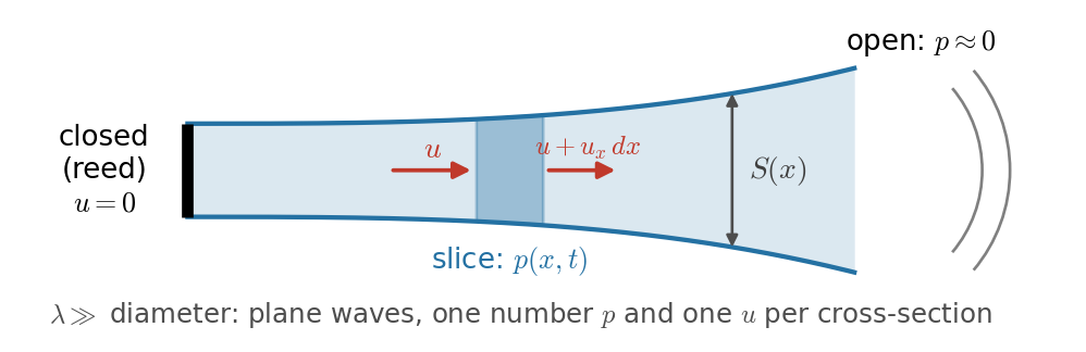
Pressure \(p(x,t)\), volume velocity \(u(x,t)\), area \(S(x)\): \[ \frac{S}{\rho c^2}\,p_t=-u_x,\qquad \frac{\rho}{S}\,u_t=-p_x \] (mass and momentum; the same form as a transmission line). With \(p=\rho\Psi_t\), \(u=-S\Psi_x\), Webster’s equation: \[ S\,\Psi_{tt}=c^2\left(S\,\Psi_x\right)_x \]

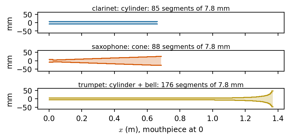
  • Cylinder (\(S\) constant): the 1D wave equation.
  • Cone (\(S\propto(x+x_0)^2\)): \(\sqrt{S}\,\Psi\) obeys the 1D wave equation (spherical waves).
  • Wave impedance \(Z_0=\rho c/S\): narrow tube, high impedance.
  • Ends: closed \(u=0\), open \(p\approx0\); really a radiation condition (lossy, mass-like) that we will replace by a reflection filter.

Show code
bores = {"clarinet: cylinder": (cylinder(**CLAR), COL["cyl"]),
         "saxophone: cone": (saxophone(), COL["cone"]),
         "trumpet: cylinder + bell": (trumpet(), COL["brass"])}
fig, axs = plt.subplots(3, 1, figsize=(5.0, 2.5), sharex=True)
for ax, (name, (S, col)) in zip(axs, bores.items()):
    x = np.arange(len(S) + 1) * dx; r = 1e3 * np.sqrt(np.r_[S, S[-1]] / np.pi)
    ax.fill_between(x, -r, r, step="post", color=col, alpha=0.25, lw=0)
    ax.step(x, r, where="post", color=col, lw=1.2); ax.step(x, -r, where="post", color=col, lw=1.2)
    ax.set_title(f"{name}: {len(S)} segments of {1e3 * dx:.1f} mm", fontsize=8, pad=2)
    ax.set_ylabel("mm"); ax.set_ylim(-62, 62)
axs[-1].set_xlabel("$x$ (m), mouthpiece at 0")
plt.tight_layout()
plt.show()

Traveling Pressure Waves in Two Delay Lines

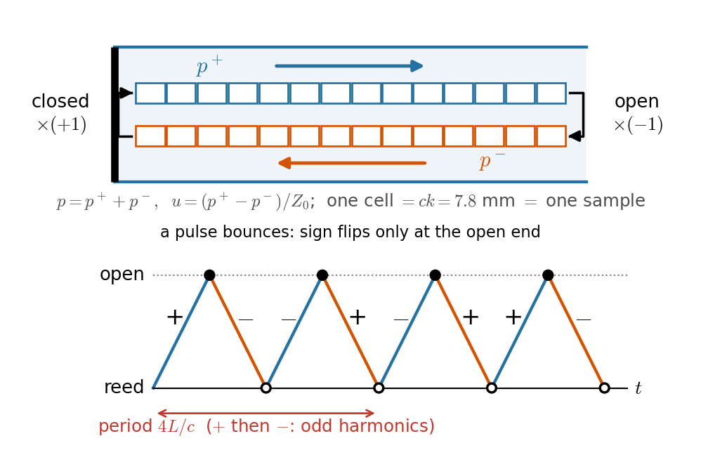
d’Alembert in pressure waves: \[ p=p^++p^-,\qquad u=\frac{p^+-p^-}{Z_0} \]

  • Closed end (\(u=0\)): \(p^-=+p^+\), reflect with \(+1\).
  • Open end (\(p=0\)): \(p^-=-p^+\), reflect with \(-1\).
  • Each delay line holds \(M=L/(ck)\) samples.
fwd, bwd = np.zeros(M), np.zeros(M)   # p+ and p-
fwd[0] = 1.0                          # a pulse at the mouthpiece
for n in range(steps):
    a, b = fwd[-1], bwd[0]            # arriving at the two ends
    fwd = np.r_[+b, fwd[:-1]]         # closed: reflect +1
    bwd = np.r_[bwd[1:], -a]          # open:   reflect -1
    out[n] = fwd[0] + bwd[0]          # pressure at the mouthpiece

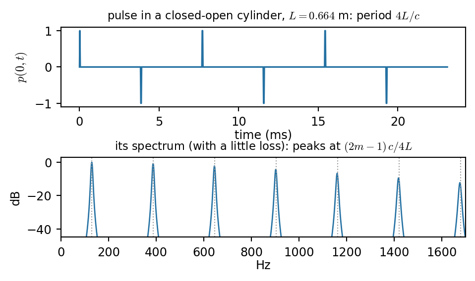
Period \(4L/c\), sign flips every half period: odd harmonics only.

Show code
S = cylinder(**CLAR); M = len(S)
bo = Bore(S, end_a=0.0); n_ = 6 * 2 * M; p0 = np.zeros(n_)
for n in range(n_):                                   # closed mouthpiece: reflect +1, plus one pulse
    p0[n] = bo.f[0] + bo.b[0]
    bo.step(bo.b[0] + (1.0 if n == 0 else 0.0))
fig = plt.figure(figsize=(5.0, 2.8))
ax = fig.add_axes([0.12, 0.62, 0.85, 0.3])
ax.plot(1e3 * np.arange(n_) * k, p0, color=COL["cyl"], lw=1.2)
ax.set_xlabel("time (ms)", labelpad=1); ax.set_yticks([-1, 0, 1]); ax.set_ylabel("$p(0,t)$")
ax.set_title(f"pulse in a closed-open cylinder, $L={CLAR['L']}$ m: period $4L/c$", fontsize=8.5)
ax = fig.add_axes([0.12, 0.13, 0.85, 0.3])
bo = Bore(S, **LOSSY); h = np.zeros(1 << 14)
for n in range(len(h)):
    h[n] = bo.f[0] + bo.b[0]; bo.step(bo.b[0] + (1.0 if n == 0 else 0.0))
f, Hd = spectrum_db(h, n=len(h))
ax.plot(f, Hd, color=COL["cyl"], lw=1)
for m in range(1, 8):
    ax.axvline((2 * m - 1) * c0 / (4 * CLAR["L"]), color="0.6", ls=":", lw=0.8)
ax.set_xlim(0, 1700); ax.set_ylim(-45, 3); ax.set_xlabel("Hz", labelpad=1); ax.set_ylabel("dB")
ax.set_title("its spectrum (with a little loss): peaks at $(2m-1)\\,c/4L$", fontsize=8.5)
plt.show()

Lumping Loss into One Loop Filter

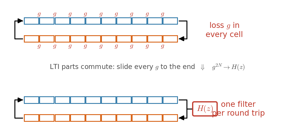
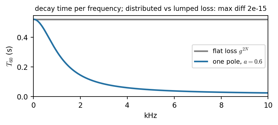
Wall friction and heat loss act everywhere, more at high frequencies. But every element is linear and time invariant, so they commute: slide them along the delay lines and collect them at one point.

  • \(2N\) factors \(g\) become one \(g^{2N}\); frequency dependent loss and radiation become one filter \(H(z)\) per round trip: \[ H(z)=g\,\frac{1-a}{1-a z^{-1}} \]
  • Stable iff \(|H(e^{j\omega})|\le1\) (a passive loop): no CFL.
  • Decay per round trip \(|H|\), so \[T_{60}(f)=\frac{3\ln10\;T_{\text{rt}}}{-\ln|H(e^{j\omega})|}\]

Show code
def tap(bore, n, mouth=False):                        # strike the closed mouthpiece once
    y = np.zeros(n)
    for i in range(n):
        p0 = bore.b[0]                                 # wave arriving at the mouthpiece
        y[i] = bore.step(bore.b[0] + (1.0 if i == 0 else 0.0))
        y[i] = p0 if mouth else y[i]
    return y
S = cylinder(**CLAR); N = len(S); g = 0.9997
same = np.abs(tap(Bore(S, loss=g, end_a=0), 8000, True) - tap(Bore(S, end_a=0, end_g=g**(2 * N)), 8000, True)).max()
y_flat = tap(Bore(S, end_a=0, end_g=g**(2 * N)), int(1.5 * fs))
y_lp = tap(Bore(S, end_a=0.6, end_g=g**(2 * N)), int(1.5 * fs))
save_wav("tap_flat", y_flat); save_wav("tap_loopfilter", y_lp)
fig, ax = plt.subplots(figsize=(5.0, 2.3))
Trt = 2 * N / fs; w = np.linspace(1e-3, np.pi, 800); f = w * fs / (2 * np.pi)
for a_, col, lab in [(0.0, "0.5", "flat loss $g^{2N}$"), (0.6, COL["cyl"], "one pole, $a=0.6$")]:
    Hm = g**(2 * N) * (1 - a_) / np.abs(1 - a_ * np.exp(-1j * w))
    ax.plot(f / 1e3, 3 * np.log(10) * Trt / -np.log(Hm), color=col, lw=2, label=lab)
ax.set_xlabel("kHz"); ax.set_ylabel("$T_{60}$ (s)"); ax.set_xlim(0, 10); ax.set_ylim(0, None); ax.legend(fontsize=8)
ax.set_title(f"decay time per frequency; distributed vs lumped loss: max diff {same:.0e}", fontsize=8.5)
plt.tight_layout()
plt.show()

flat loss (all partials alike)

loop filter (highs die first)

Fractional Delay: Tuning the Loop

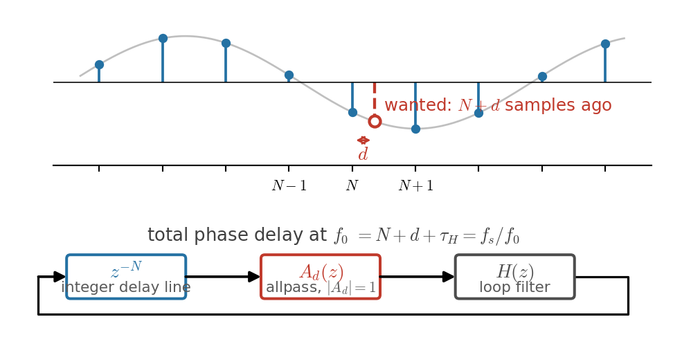
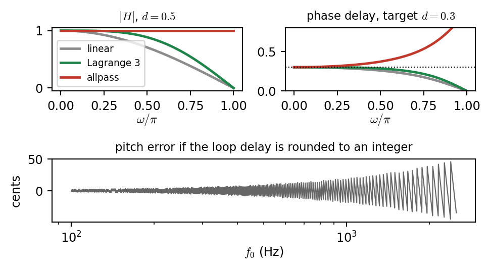
Loop delay must equal one period \(f_s/f_0\), not an integer. Delay \(d\in[0,1)\) samples by interpolation (class 8):

filter \(\lvert H\rvert\)
linear \((1-d)+d\,z^{-1}\) lowpass, \(0\) at Nyquist if \(d=\tfrac12\)
Lagrange 3 4 taps flatter, still \(<1\)
allpass \(\frac{\eta+z^{-1}}{1+\eta z^{-1}}\) exactly 1
  • Linear: timbre changes from note to note.
  • Allpass, \(\eta=\frac{1-d}{1+d}\): lossless, ideal inside a loop; click if \(d\) jumps.
  • The loop filter adds delay too: subtract its phase delay at \(f_0\).
D = fs / f0 - pd_lp - pd_dc     # delay line length
Ni = int(np.floor(D - 0.1)); d = D - Ni
eta = (1 - d) / (1 + d)
y = eta * x + x_prev - eta * y_prev   # allpass

C6 to C7, integer delays

allpass fractional delay

Show code
w = np.linspace(1e-3, np.pi, 600); z1 = np.exp(-1j * w)
def lagrange3(d):                                     # taps for delay 1 + d (centered), returns (filter, extra delay)
    D_ = 1 + d; n_ = np.arange(4)
    return np.array([np.prod([(D_ - m) / (n - m) for m in n_ if m != n]) for n in n_]), 1
filt = {"linear": lambda d: ((1 - d) + d * z1, 0), "Lagrange 3": lambda d: (np.polyval(lagrange3(d)[0][::-1], z1), 1),
        "allpass": lambda d: (((1 - d) / (1 + d) + z1) / (1 + (1 - d) / (1 + d) * z1), 0)}
cols = {"linear": "0.55", "Lagrange 3": COL["flute"], "allpass": COL["exciter"]}
fig, axs = plt.subplots(2, 2, figsize=(5.2, 2.9))
for name, F in filt.items():
    H, extra = F(0.5); axs[0, 0].plot(w / np.pi, np.abs(H), color=cols[name], lw=1.8, label=name)
    H, extra = F(0.3); axs[0, 1].plot(w / np.pi, -np.unwrap(np.angle(H)) / w - extra, color=cols[name], lw=1.8)
axs[0, 0].set_title("$|H|$, $d=0.5$", fontsize=8.5); axs[0, 0].legend(fontsize=7)
axs[0, 1].axhline(0.3, color="k", ls=":", lw=0.8); axs[0, 1].set_ylim(0, 0.8)
axs[0, 1].set_title("phase delay, target $d=0.3$", fontsize=8.5)
for ax in axs[0]:
    ax.set_xlabel("$\\omega/\\pi$", labelpad=0)
gs = axs[1, 0].get_gridspec(); axs[1, 0].remove(); axs[1, 1].remove()
ax = fig.add_subplot(gs[1, :])
f0s = np.geomspace(100, 2500, 2000); D_ = fs / f0s
ax.plot(f0s, 1200 * np.log2(D_ / np.round(D_)), color="0.4", lw=0.8)
ax.set_xscale("log"); ax.set_xlabel("$f_0$ (Hz)", labelpad=0); ax.set_ylabel("cents")
ax.set_title("pitch error if the loop delay is rounded to an integer", fontsize=8.5)
plt.tight_layout()
plt.show()
scale = 1046.5 * 2**(np.array([0, 2, 4, 5, 7, 9, 11, 12]) / 12)
for name, frac in [("int", False), ("frac", True)]:
    save_wav(f"scale_{name}", np.concatenate([flute(f, 1.0, dur=0.32, frac=frac, noise=0.02, seed=j) for j, f in enumerate(scale)]))
Junctions: Scattering at an Area Change

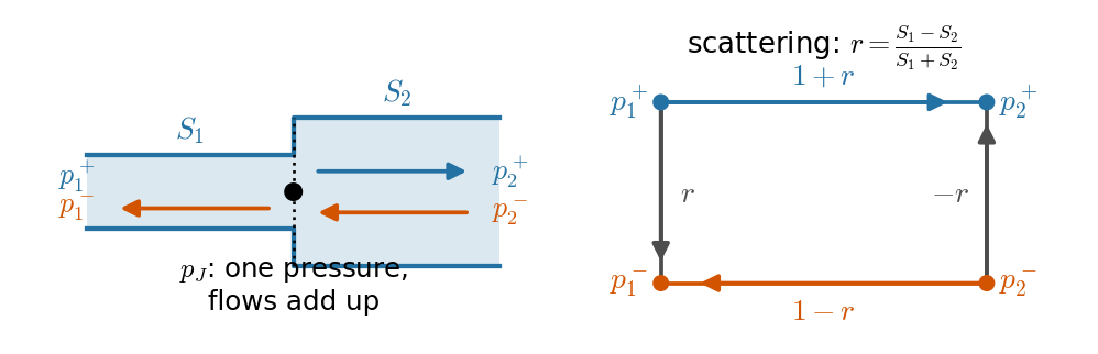
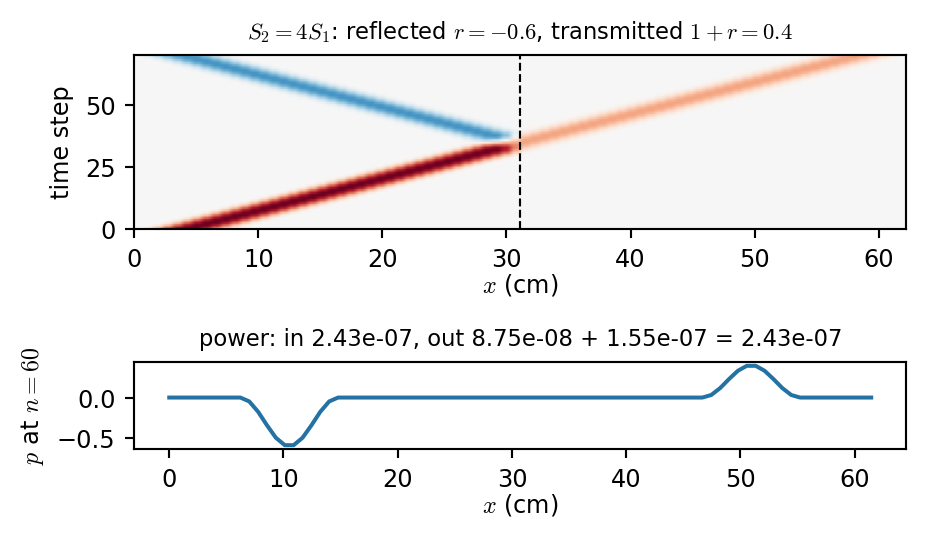
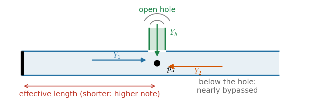
Two cylinders meet: one pressure, flows add up. With admittances \(Y_i=S_i/\rho c\): \[ p_J=\frac{2\,(Y_1p_1^++Y_2p_2^-)}{Y_1+Y_2},\qquad p^{\text{out}}_i=p_J-p^{\text{in}}_i \] Equivalently, a reflection coefficient \[ r=\frac{S_1-S_2}{S_1+S_2}\quad\begin{cases}r\to-1 & S_2\to\infty\ \text{(open)}\\ r\to+1 & S_2\to0\ \text{(closed)}\end{cases} \]

pJ = 2 * (Y[:-1] * f[:-1] + Y[1:] * b[1:]) / (Y[:-1] + Y[1:])
f[1:], b[:-1] = pJ - b[1:], pJ - f[:-1]    # then shift
  • Power in = power out (\(Y p^2\) per wave): lossless, so any network of junctions is stable.
  • A junction at every segment: the Kelly–Lochbaum tube (1962), the first physical model of the voice.

Show code
S = np.r_[np.full(40, 1e-4), np.full(40, 4e-4)]       # the area jumps by 4 at x = 40 segments
bo = Bore(S, end_a=0.0, end_g=0.0); nt = 70; P = np.zeros((nt, len(S)))
bo.f[:12] = np.hanning(12)                             # a right going pulse
for n in range(nt):
    P[n] = bo.f + bo.b; bo.step(0.0)
r_ = (S[0] - S[-1]) / (S[0] + S[-1])
inc, refl, trans = bo.Y[0] * 1, bo.Y[0] * r_**2, bo.Y[-1] * (1 + r_)**2
fig, axs = plt.subplots(2, 1, figsize=(4.9, 2.9), height_ratios=[2, 1])
axs[0].imshow(P, aspect="auto", origin="lower", cmap="RdBu_r", vmin=-1, vmax=1, extent=[0, len(S) * dx * 100, 0, nt])
axs[0].axvline(40 * dx * 100, color="k", lw=0.8, ls="--")
axs[0].set_xlabel("$x$ (cm)", labelpad=0); axs[0].set_ylabel("time step")
axs[0].set_title(f"$S_2=4S_1$: reflected $r={r_:.1f}$, transmitted $1+r={1 + r_:.1f}$", fontsize=8.5)
axs[1].plot(np.arange(len(S)) * dx * 100, P[60], color=COL["cyl"], lw=1.5)
axs[1].set_xlabel("$x$ (cm)", labelpad=0); axs[1].set_ylabel("$p$ at $n=60$")
axs[1].set_title(f"power: in {inc:.3g}, out {refl:.3g} + {trans:.3g} = {refl + trans:.3g}", fontsize=8.5)
plt.tight_layout()
plt.show()

Kelly–Lochbaum as a Finite Difference

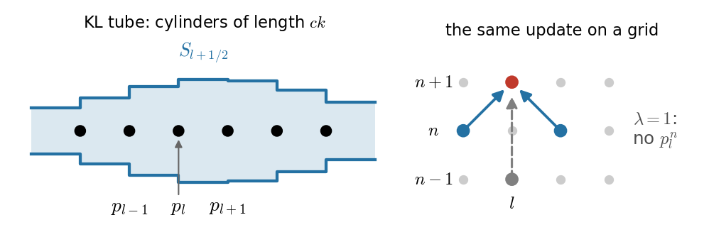
Eliminate the waves from scatter + shift: the junction pressures obey \[ p_l^{n+1}=\frac{2\,(S_{l+\frac12}\,p_{l+1}^n+S_{l-\frac12}\,p_{l-1}^n)}{S_{l-\frac12}+S_{l+\frac12}}-p_l^{n-1} \]

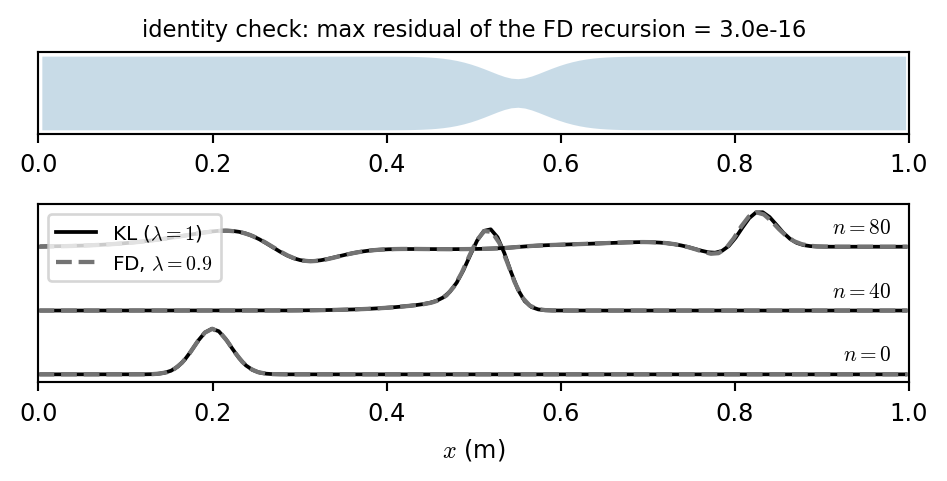
which is the finite difference scheme for Webster’s equation \[ [\mu_{xx}S]\,\delta_{tt}p=c^2\,\delta_{x+}\big((\mu_{x-}S)\,\delta_{x-}p\big) \] at \(\lambda=ck/h=1\) (the \(p_l^n\) term drops out, as for the string in class 14).

waveguide (KL) finite differences
grid \(h=ck\) fixed any \(h\), \(\lambda\le1\)
tuning fractional delay choose \(h\)
extra terms (wall, nonlinear) hard natural
dispersion none from the scheme small for tubes
Show code
rng = np.random.default_rng(0)
S = np.exp(rng.uniform(-1, 1, 30)) * 1e-4; bo = Bore(S, end_a=0.0)
bo.f, bo.b = rng.standard_normal(30), rng.standard_normal(30)
PJ = []
for n in range(40):                                   # junction pressures of the KL tube, j = 0 .. 28
    PJ.append(2 * (bo.Y[:-1] * bo.f[:-1] + bo.Y[1:] * bo.b[1:]) / (bo.Y[:-1] + bo.Y[1:])); bo.step(0.0)
PJ = np.array(PJ); Sl, Sr = S[1:-2], S[2:-1]          # junction j: segment j on its left, j + 1 on its right
fd = 2 * (Sr * PJ[1:-1, 2:] + Sl * PJ[1:-1, :-2]) / (Sl + Sr) - PJ[:-2, 1:-1]
res = np.abs(fd - PJ[2:, 1:-1]).max() / np.abs(PJ).max()

L_, Nk = 1.0, 128; xk = (np.arange(Nk) + 0.5) / Nk * L_      # a tube with a constriction, KL vs FD at lambda = 0.9
Sx = lambda x: 1e-4 * (1 - 0.85 * np.exp(-((x - 0.55) / 0.06)**2))
pulse = lambda x: np.exp(-((x - 0.2) / 0.03)**2)
bo = Bore(Sx(xk), end_a=0.0); bo.f[:] = pulse(xk); snaps_kl = []
lam = 0.9; h = c0 * k / lam * (L_ / (Nk * dx)); Nf = int(L_ / h); xf = np.arange(Nf + 1) * h
Sm = Sx(np.r_[xf, xf[-1] + h] - h / 2)                 # S at half points (mu_x- S)
Sj = 0.5 * (Sm[:-1] + Sm[1:])                          # [mu_xx S] at the nodes
ct = c0 * (L_ / (Nk * dx))                             # same travel time per meter as the KL tube
p = pulse(xf); pp = pulse(xf + ct * k)                 # right going: p^{-1}(x) = p^0(x + c k)
snaps_fd = []
T_ = [0, 40, 80]
for n in range(81):
    if n in T_:
        snaps_kl.append(bo.f + bo.b); snaps_fd.append(p.copy())
    bo.step(0.0)
    lap = np.zeros_like(p)
    lap[1:-1] = (Sm[2:-1] * (p[2:] - p[1:-1]) - Sm[1:-2] * (p[1:-1] - p[:-2]))
    pn = 2 * p - pp + (ct * k / h)**2 * lap / Sj; pn[0] = pn[-1] = 0; pp, p = p, pn
fig, axs = plt.subplots(2, 1, figsize=(5.0, 2.6), height_ratios=[1, 2.2])
axs[0].fill_between(xk, -np.sqrt(Sx(xk) / 1e-4), np.sqrt(Sx(xk) / 1e-4), color=COL["cyl"], alpha=0.25, lw=0)
axs[0].set_yticks([]); axs[0].set_title(f"identity check: max residual of the FD recursion = {res:.1e}", fontsize=8.5)
for i, n in enumerate(T_):
    axs[1].plot(xk, snaps_kl[i] + 1.4 * i, color="k", lw=1.4, label="KL ($\\lambda=1$)" if i == 0 else None)
    axs[1].plot(xf, snaps_fd[i] + 1.4 * i, color=COL["fd"], lw=1.6, ls="--", label="FD, $\\lambda=0.9$" if i == 0 else None)
    axs[1].text(0.98, 1.4 * i + 0.3, f"$n={n}$", fontsize=8, ha="right")
axs[1].set_yticks([]); axs[1].set_xlabel("$x$ (m)"); axs[1].legend(fontsize=7.5, loc="upper left")
for ax in axs:
    ax.set_xlim(0, 1)
plt.tight_layout()
plt.show()

In 2D: The Waveguide Mesh

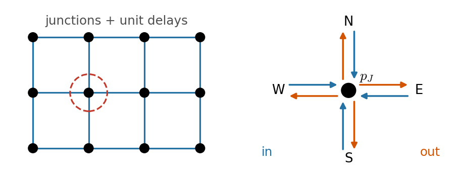
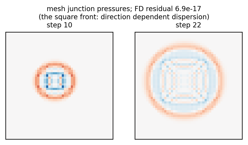
Four-port junctions on a grid, unit delays between them: \[ p_J=\tfrac12\sum_{\text{N,S,E,W}}p^{\text{in}},\qquad p^{\text{out}}=p_J-p^{\text{in}} \] Eliminating the waves gives the 2D wave scheme of class 15 at \(\lambda=1/\sqrt2\): \[ p_{l,m}^{n+1}=\tfrac12\left(p_{l\pm1,m}^n+p_{l,m\pm1}^n\right)-p_{l,m}^{n-1} \]

per grid point mesh FD
memory 5 2
operations 8 5
per sample \(O(N^2)\) \(O(N^2)\)

The \(O(1)\) delay line trick is a 1D privilege; the mesh keeps only structural stability (passive junctions).

Show code
Nm = 48; W = {d: np.zeros((Nm, Nm)) for d in "NSEW"}  # waves arriving at each junction from N, S, E, W
W["N"][20:24, 20:24] = 0.5; W["S"][20:24, 20:24] = 0.5; PJ = []
for n in range(60):
    pJ = 0.5 * (W["N"] + W["S"] + W["E"] + W["W"]); PJ.append(pJ)
    out = {d: pJ - W[d] for d in "NSEW"}               # scatter
    W = {"N": np.zeros_like(pJ), "S": np.zeros_like(pJ), "E": np.zeros_like(pJ), "W": np.zeros_like(pJ)}
    W["S"][1:] = out["N"][:-1]; W["N"][:-1] = out["S"][1:]    # shift to the neighbors (rigid walls: lost at the rim)
    W["W"][:, 1:] = out["E"][:, :-1]; W["E"][:, :-1] = out["W"][:, 1:]
PJ = np.array(PJ)
fd = 0.5 * (PJ[1:-1, 2:, 1:-1] + PJ[1:-1, :-2, 1:-1] + PJ[1:-1, 1:-1, 2:] + PJ[1:-1, 1:-1, :-2]) - PJ[:-2, 1:-1, 1:-1]
res = np.abs(fd - PJ[2:, 1:-1, 1:-1]).max()
fig, axs = plt.subplots(1, 2, figsize=(4.6, 2.5))
for ax, n in zip(axs, [10, 22]):
    ax.imshow(PJ[n], cmap="RdBu_r", vmin=-0.3, vmax=0.3); ax.set_xticks([]); ax.set_yticks([])
    ax.set_title(f"step {n}", fontsize=8.5)
fig.suptitle(f"mesh junction pressures; FD residual {res:.1e}\n(the square front: direction dependent dispersion)", fontsize=8.5)
plt.tight_layout()
plt.show()

The Bore as a Resonator

Input Impedance: The Peaks Are the Notes

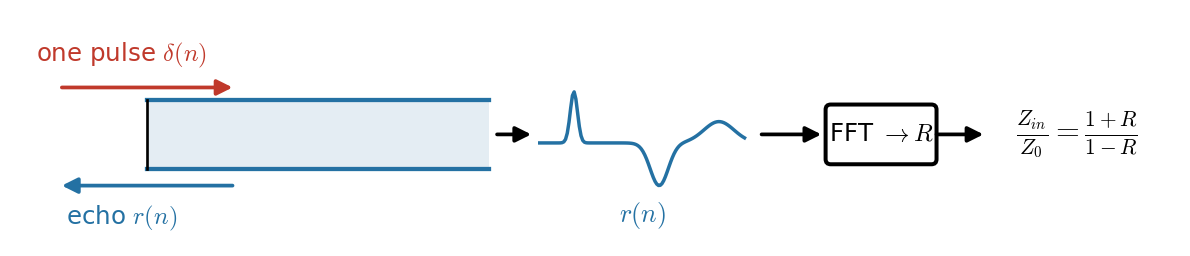
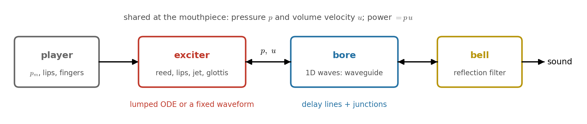
What the exciter sees: pressure per unit flow at the mouthpiece.

  1. Send one pulse in; record what comes back: the reflection function \(r(n)\) (the bore’s impulse response).
  2. \(Z_{\text{in}}(\omega)=Z_0\,\dfrac{1+R(\omega)}{1-R(\omega)}\).

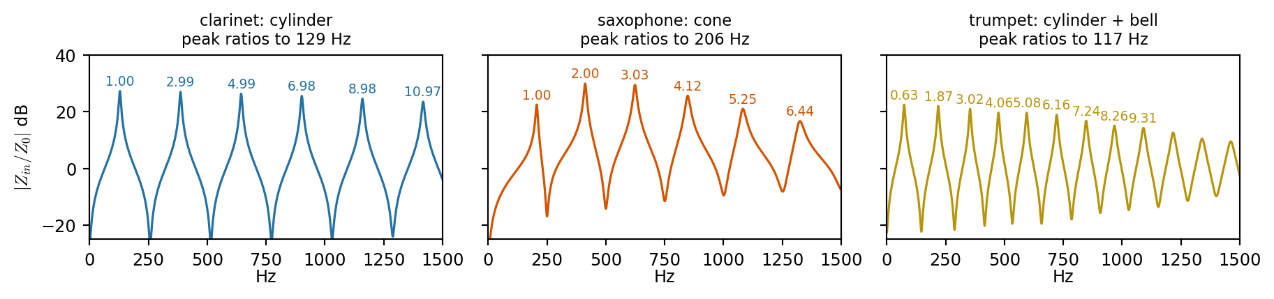
A pressure controlled valve (reed, lips) oscillates where the pressure can swing: at the impedance peaks. They are the playable notes.

  • Cylinder: \(1,3,5,\dots\) (closed-open)
  • Cone: \(1,2,3,\dots\) (like open-open)
  • Cylinder + bell: odd peaks pulled into a harmonic series

Show code
fig, axs = plt.subplots(1, 3, figsize=(9.6, 2.3), sharey=True)
for ax, (name, (S, col)) in zip(axs, bores.items()):
    f, Z = input_impedance(S, n=1 << 15, **LOSSY)
    a = 20 * np.log10(np.abs(Z)); ax.plot(f, a, color=col, lw=1.2)
    pk = peaks_of(f, a, 1500, thr=0)
    base = pk[0] if "trumpet" not in name else np.mean(pk[1:6] / np.arange(2, 7))
    for j, fp in enumerate(pk[:9]):
        ax.text(fp, a[np.argmin(np.abs(f - fp))] + 2, f"{fp / base:.2f}", fontsize=7, ha="center", color=col)
    ax.set_ylim(-25, 40); ax.set_xlim(0, 1500); ax.set_xlabel("Hz", labelpad=0)
    ax.set_title(f"{name}\npeak ratios to {base:.0f} Hz", fontsize=8.5)
axs[0].set_ylabel("$|Z_{in}/Z_0|$ dB")
plt.tight_layout()
plt.show()

Cylinders and Cones

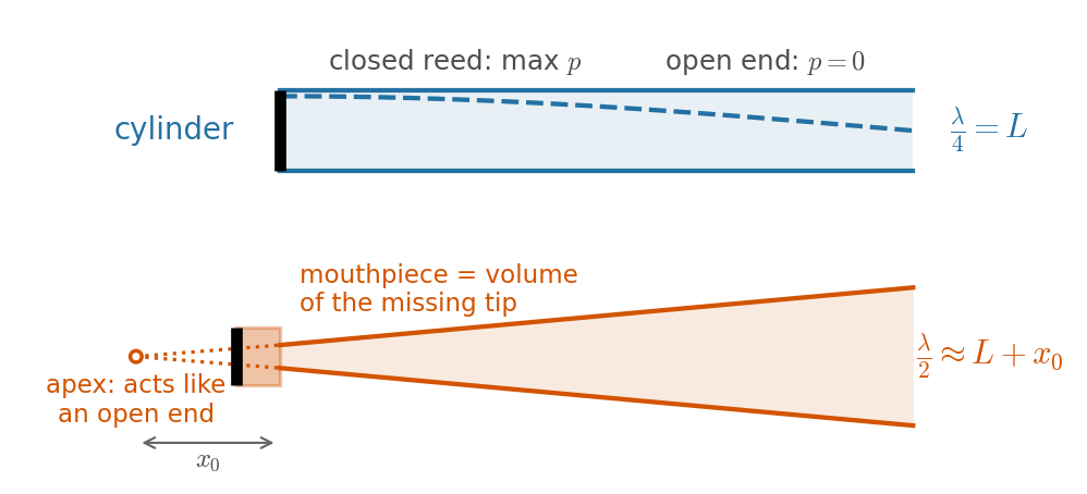
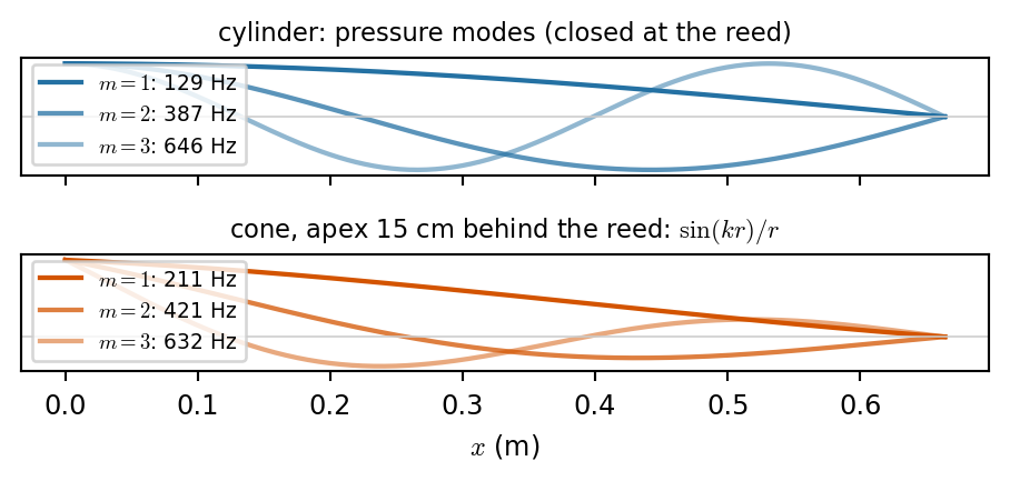
Cylinder, closed at the reed, open at the end: \(p_m(x)\propto\cos(k_mx)\) with \(\cos(k_mL)=0\): \[ f_m=(2m-1)\,\frac{c}{4L} \] odd harmonics; overblows by a twelfth (clarinet).

Two waveguide options for a cone:

  • delay lines in \(r\,p\) + a filter at the truncated apex,
  • Kelly–Lochbaum steps (today): the same code, only \(S\) changes; cost \(O(N)\) per sample. The missing apex is replaced by a short wide mouthpiece of the same volume.

Cone with apex at \(r=0\): \(r\,p\) obeys the 1D wave equation and must vanish at the apex, so \(p_m(r)\propto\dfrac{\sin(k_mr)}{r}\): \[ f_m\approx m\,\frac{c}{2(L+x_0)} \] all harmonics; overblows by an octave (saxophone, oboe, bassoon).

Show code
L_, x0 = 0.664, 0.15; x = np.linspace(0, L_, 400)
fig, axs = plt.subplots(2, 1, figsize=(4.8, 2.35), sharex=True)
for m in range(1, 4):
    km = (2 * m - 1) * np.pi / (2 * L_)
    axs[0].plot(x, np.cos(km * x), color=COL["cyl"], lw=1.6, alpha=1 - 0.25 * (m - 1),
                label=f"$m={m}$: {(2 * m - 1) * c0 / (4 * L_):.0f} Hz")
for m in range(1, 4):
    kr = np.pi * m / (L_ + x0); r = x + x0          # p = 0 at the open end: sin(k (L + x0)) = 0
    p = np.sin(kr * r) / r; p /= np.abs(p).max()
    axs[1].plot(x, p, color=COL["cone"], lw=1.6, alpha=1 - 0.25 * (m - 1), label=f"$m={m}$: {m * c0 / (2 * (L_ + x0)):.0f} Hz")
axs[0].set_title("cylinder: pressure modes (closed at the reed)", fontsize=8.5)
axs[1].set_title(f"cone, apex {100 * x0:.0f} cm behind the reed: $\\sin(kr)/r$", fontsize=8.5)
for ax in axs:
    ax.axhline(0, color="0.8", lw=0.6); ax.legend(fontsize=7, loc="lower left"); ax.set_yticks([])
axs[1].set_xlabel("$x$ (m)")
plt.tight_layout()
plt.show()

The Bell: A Frequency Dependent Reflection

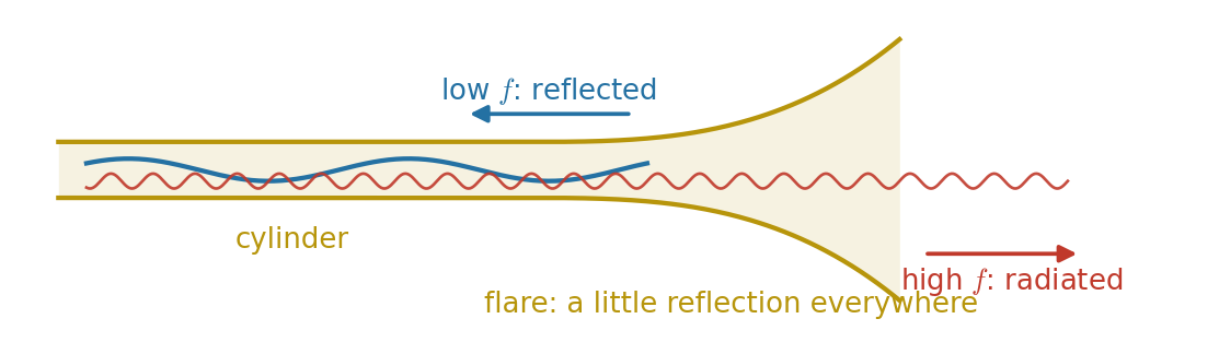
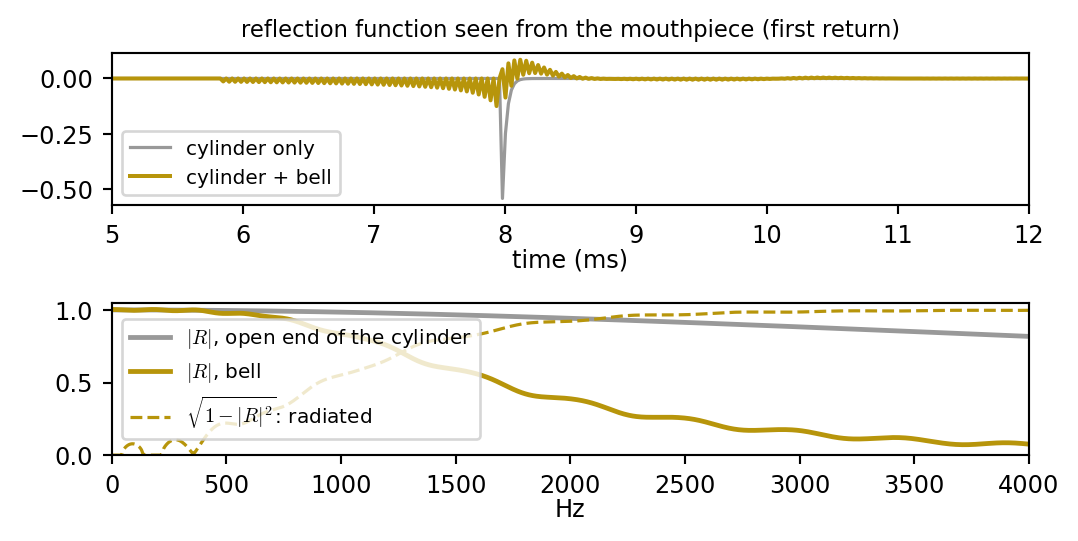
The flare reflects a little everywhere, so the reflection is spread out in time and depends on frequency:

  • Low frequencies: reflected (they see the flare as an abrupt end).
  • High frequencies: transmitted (the flare is gradual on their scale).
  • \(|R|^2+|T|^2=1\): a lowpass reflector is a highpass radiator: bright brass tone, and no impedance peaks up high.

Two ways in a waveguide:

  1. the flare as KL steps (today), or
  2. a reflection filter fitted to \(r(n)\) (or measured) at the end of a plain cylinder: cheap and common in real time.

Show code
St = trumpet(); Sc = np.full(len(St), St[0])
r_t = reflectance(St, n=1 << 13)                     # open end filter scaled by the end radius
r_c = reflectance(Sc, n=1 << 13)
fig, axs = plt.subplots(2, 1, figsize=(5.6, 2.9))
t_ms = 1e3 * np.arange(len(r_t)) * k
axs[0].plot(t_ms, r_c, color="0.6", lw=1.2, label="cylinder only")
axs[0].plot(t_ms, r_t, color=COL["brass"], lw=1.5, label="cylinder + bell")
axs[0].set_xlim(5, 12); axs[0].set_xlabel("time (ms)", labelpad=0); axs[0].legend(fontsize=7.5)
axs[0].set_title("reflection function seen from the mouthpiece (first return)", fontsize=8.5)
win = (np.arange(len(r_t)) < int(0.0125 * fs))         # first return only
for r_, col, lab in [(r_c, "0.6", "open end of the cylinder"), (r_t, COL["brass"], "bell")]:
    R = np.fft.rfft(r_ * win); f = np.fft.rfftfreq(len(r_), k)
    axs[1].plot(f, np.abs(R), color=col, lw=1.8, label=f"$|R|$, {lab}")
    if col != "0.6":
        axs[1].plot(f, np.sqrt(np.maximum(0, 1 - np.abs(R)**2)), color=col, lw=1.2, ls="--", label="$\\sqrt{1-|R|^2}$: radiated")
axs[1].set_xlim(0, 4000); axs[1].set_ylim(0, 1.05); axs[1].set_xlabel("Hz", labelpad=0); axs[1].legend(fontsize=7.5)
plt.tight_layout()
plt.show()

Toneholes: A Three-Port Junction

A tonehole is a short side tube: three tubes meet at one pressure, and the three flows sum to zero: \[ p_J=\frac{2\,(Y_1p_1^{\text{in}}+Y_2p_2^{\text{in}}+Y_hp_h^{\text{in}})}{Y_1+Y_2+Y_h} \] \(p^{\text{out}}_i=p_J-p^{\text{in}}_i\), with \(Y_h=S_h/\rho c\).

  • Hole = a few samples of delay line, reflected with \(-1\) at its open end; closed: branch removed (\(Y_h=0\)).
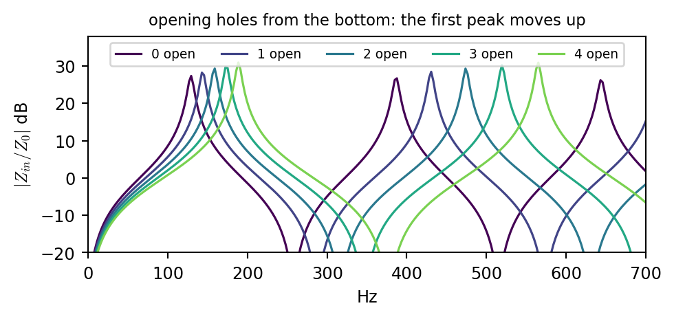
  • A big open hole cuts the bore: the effective length shrinks and the pitch rises.
num[j] += Yh * h_in; den[j] += Yh   # one extra term

Show code
S = cylinder(**CLAR); a_h = 0.0055; Yh = np.pi * a_h**2 / (rho * c0)
pos = [0.425, 0.465, 0.51, 0.57]                       # hole positions (m), top to bottom
def holes(n_open):                                     # open the lowest n_open holes
    return [dict(j=int(round(x / dx)), Yh=Yh, D=4, open=(i >= len(pos) - n_open)) for i, x in enumerate(pos)]
fig, ax = plt.subplots(figsize=(5.2, 2.5))
for m in range(5):
    bo = Bore(S, **LOSSY, holes=holes(m)); r_ = np.zeros(1 << 14)
    for i in range(len(r_)):
        r_[i] = bo.b[0]; bo.step(1.0 if i == 0 else 0.0)
    R = np.fft.rfft(r_); f = np.fft.rfftfreq(len(r_), k)
    ax.plot(f, 20 * np.log10(np.abs((1 + R) / (1 - R))), color=plt.cm.viridis(m / 5), lw=1.2, label=f"{m} open")
ax.set_xlim(0, 700); ax.set_ylim(-20, 38); ax.set_xlabel("Hz"); ax.set_ylabel("$|Z_{in}/Z_0|$ dB")
ax.legend(fontsize=7, ncol=5, loc="upper center"); ax.set_title("opening holes from the bottom: the first peak moves up", fontsize=8.5)
plt.tight_layout()
plt.show()
bo = Bore(S, **LOSSY, holes=holes(0)); reed = Reed(bo.Z0); nn = int(0.42 * fs)
def finger(i):                                         # change the fingering every note
    if i % nn == 0:
        for j_, h_ in enumerate(bo.holes):
            h_["open"] = j_ >= len(pos) - (i // nn)
pm_ = lambda t: 0.6 * reed.pM * min(1, t / 0.03) * (1 - 0.5 * np.exp(-((t % 0.42) / 0.01)**2))
out_scale = play(bo, reed, pm_, dur=5 * 0.42, on_step=finger)
save_wav("tonehole_scale", out_scale["y"])
f_notes = [f0_of(out_scale["pin"][:int((m + 1) * nn)]) for m in range(5)]

clarinet, opening holes one by one: 127 · 141 · 155 · 169 · 184 Hz

Exciters using Parametric/Coupled Models

One Scalar Equation at the Mouthpiece

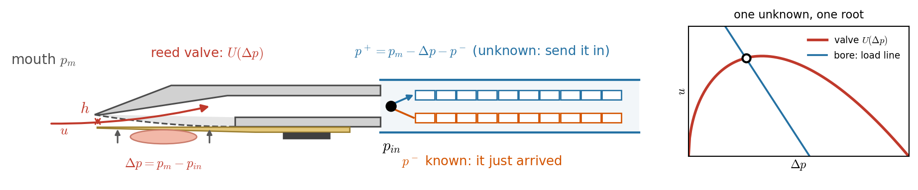
At step \(n\) the bore delivers \(p^-\) (end of a delay line). Unknown: \(p^+\).

Bore side (the waves): \(p_{\text{in}}=p^++p^-\) and \(u=(p^+-p^-)/Z_0\). With \(\Delta p=p_m-p_{\text{in}}\) this is the load line \[ u=\frac{p_m-2p^--\Delta p}{Z_0} \] Exciter side: the valve lets through \(U(\Delta p,\ \text{state})\).

Equate the two: one scalar equation for \(\Delta p\), \[ U(\Delta p)=\frac{p_m-2p^--\Delta p}{Z_0},\qquad p^+=p_m-\Delta p-p^- \] the same shape as the bow in class 16.

exciter valve equation per step
reed closes with \(\Delta p\) table, or reed ODE + root
lips opens with \(\Delta p\) lip ODE + root
flute jet none: jet deflected, delayed explicit (delay + sigmoid)
glottis prescribed flow none (one-way)

Parametric is enough when…

  • the exciter impedance \(\gg Z_0\): the source does not listen (voice);
  • the exciter resonance \(\gg f_0\): quasi-static, a memoryless table (most clarinet notes).

Couple the exciter ODE when you need the threshold, regime selection, beating, squeaks, or the lips’ pitch control.

A Memoryless Reed: The Reflection Table

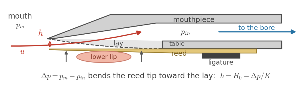
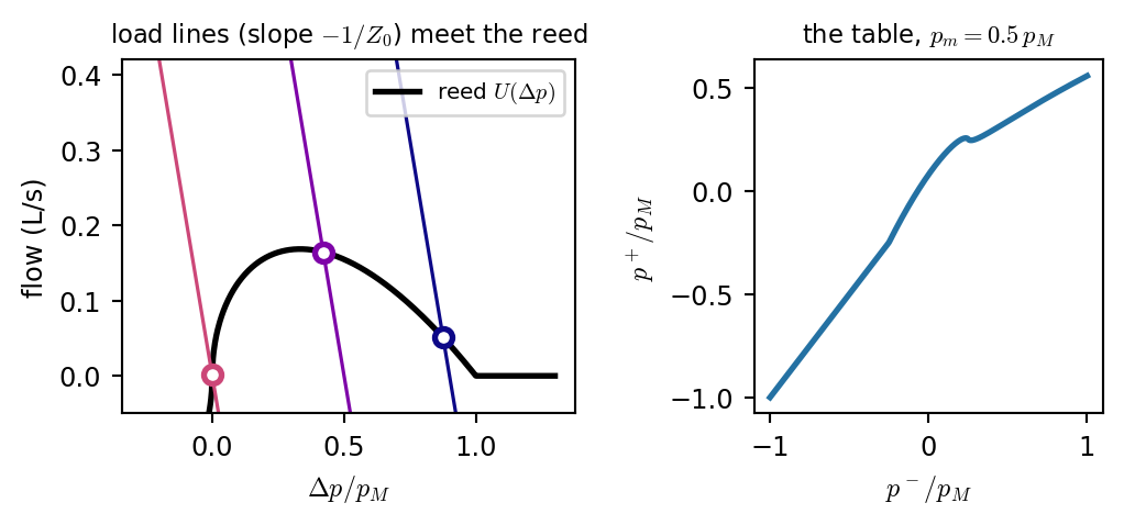
Massless reed (a spring of stiffness \(K\)): opening \(h=H_0-\Delta p/K\), closed at \(p_M=KH_0\). Bernoulli flow: \[ U(\Delta p)=w\,[h]_+\sqrt{\tfrac{2|\Delta p|}{\rho}}\,\operatorname{sgn}\Delta p \]

  • Falling branch (\(\Delta p\to p_M\)): negative resistance, the energy source (like the falling friction curve of the bow).
  • Unique root iff the load line is steeper than the falling branch: \(Z_0\max(-U')<1\).
  • The root depends on one number \(p_m-2p^-\): tabulate once, interpolate every step.
dp = np.interp(pm - 2 * pminus, tab_x, tab_d)
pplus = pm - dp - pminus

Show code
S = cylinder(**CLAR); bo = Bore(S); rt = Reed(bo.Z0, table=True); pM = rt.pM
d = np.linspace(-0.2, 1.3, 600) * pM
fig, axs = plt.subplots(1, 2, figsize=(5.4, 2.6), width_ratios=[1.3, 1])
axs[0].plot(d / pM, 1e3 * rt.u_static(d), color="k", lw=2, label="reed $U(\\Delta p)$")
for i, pminus in enumerate([-0.2, 0.0, 0.25, 0.45]):
    P = 0.5 * pM - 2 * pminus * pM
    axs[0].plot(d / pM, 1e3 * (P - d) / bo.Z0, color=plt.cm.plasma(i / 4), lw=1.2)
    ds = np.interp(P, rt.tab_x, rt.tab_d)
    axs[0].plot(ds / pM, 1e3 * rt.u_static(ds), "o", color=plt.cm.plasma(i / 4), mfc="white", mew=2)
axs[0].set_ylim(-0.05, 0.42); axs[0].set_xlabel("$\\Delta p/p_M$"); axs[0].set_ylabel("flow (L/s)")
axs[0].set_title("load lines (slope $-1/Z_0$) meet the reed", fontsize=8.5); axs[0].legend(fontsize=7.5)
pm_ = np.linspace(-1, 1, 400) * pM
axs[1].plot(pm_ / pM, (0.5 * pM - np.interp(0.5 * pM - 2 * pm_, rt.tab_x, rt.tab_d) - pm_) / pM, color=COL["cyl"], lw=2)
axs[1].set_xlabel("$p^-/p_M$"); axs[1].set_ylabel("$p^+/p_M$"); axs[1].set_title("the table, $p_m=0.5\\,p_M$", fontsize=8.5)
plt.tight_layout()
plt.show()
bo = Bore(S, **LOSSY); out_tab = play(bo, Reed(bo.Z0, table=True), 0.5 * pM, dur=1.5)
save_wav("clar_table", out_tab["y"])

clarinet = cylinder delay lines + one table, \(p_m=0.5\,p_M\) (128.9 Hz)

The Reed as a Mass-Spring

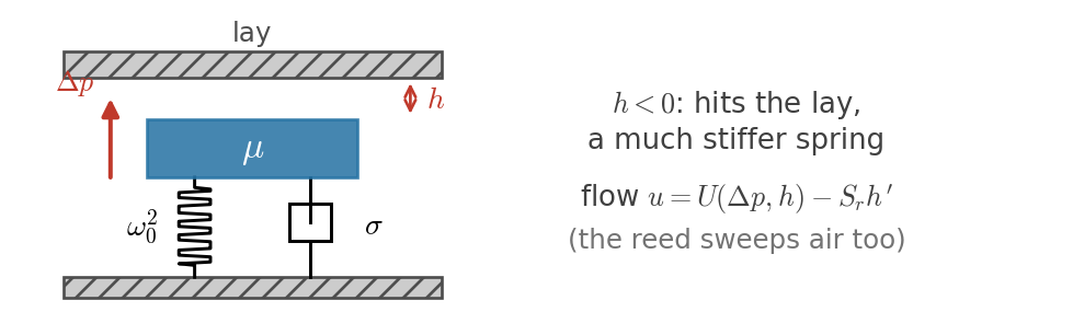
\[ h''+2\sigma h'+\omega_0^2(h-H_0)=-\frac{\Delta p}{\mu}\ \ (+\text{lay}) \] \[ u=U(\Delta p,h)-S_r\,h' \] Semi-implicit stiffness (class 13), \(\mu_{t\cdot}h\) in the spring:

  • \(h^{n+1}=A-B\,\Delta p\), \(\ \delta_{t\cdot}h=a-b\,\Delta p\): linear in \(\Delta p\).
  • Bernoulli with the known opening \(h^n\).

With \(x=\sqrt{|\Delta p|}\) the root is a quadratic: \[ D\,x^2+c_1\,x=|R| \] with \(D=\tfrac{1}{Z_0}+S_rb>0\) and \(c_1=w\,[h^n]_+\sqrt{2/\rho}\ge0\).

x = (-c1 + np.sqrt(c1**2 + 4 * D * abs(R))) / (2 * D)
dp = np.sign(R) * x**2            # unique: the left side is monotone
h_next = A - B * dp

Newton (class 5) is needed once you use \(h^{n+1}\) in Bernoulli, a general flow exponent, or air inertia in the mouthpiece.

Show code
bo = Bore(S, **LOSSY); rd = Reed(bo.Z0)
out_dyn = play(bo, rd, 0.5 * pM, dur=1.5)
save_wav("clar_dynamic", out_dyn["y"])
sl = slice(int(1.2 * fs), int(1.2 * fs) + int(3 * fs / 128))
t_ = 1e3 * np.arange(sl.stop - sl.start) * k
fig, axs = plt.subplots(2, 1, figsize=(4.9, 2.3), sharex=True)
x1, x2 = out_tab["pin"][sl], out_dyn["pin"][sl]
lag = np.argmax([np.dot(x1, np.roll(out_dyn["pin"], -j)[sl]) for j in range(int(fs / 120))])   # align the phases
for o, col, lab, lw, j in [(out_tab, "0.6", "table (memoryless)", 3, 0), (out_dyn, COL["exciter"], "mass-spring reed", 1.3, lag)]:
    axs[0].plot(t_, np.roll(o["state"], -j)[sl] / 4e-4, color=col, lw=lw, label=lab)
    axs[1].plot(t_, np.roll(o["pin"], -j)[sl] / pM, color=col, lw=lw)
axs[0].set_ylabel("$h/H_0$"); axs[0].legend(fontsize=7.5, ncol=2, loc="upper center"); axs[0].set_ylim(-0.1, 1.6)
axs[1].set_ylabel("$p_{in}/p_M$"); axs[1].set_xlabel("time (ms)")
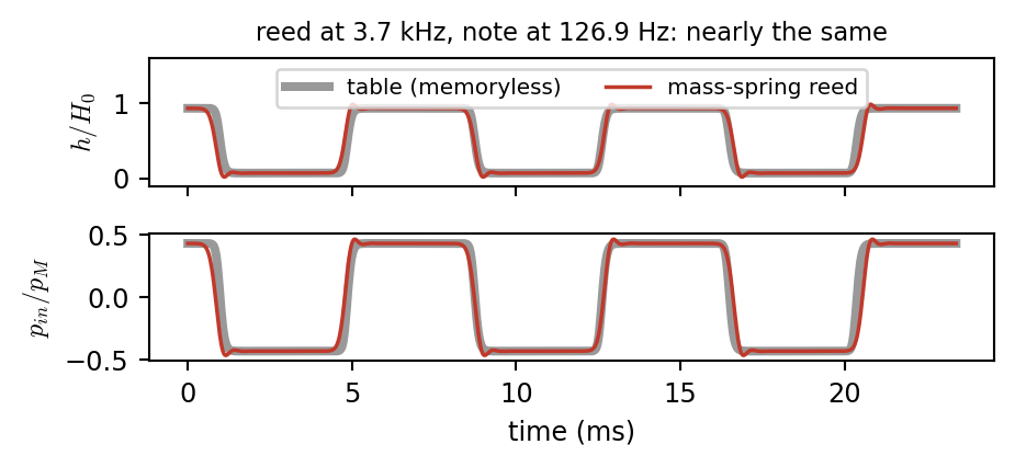
axs[0].set_title(f"reed at 3.7 kHz, note at {f0_of(out_dyn['pin']):.1f} Hz: nearly the same", fontsize=8.5)
plt.tight_layout()
plt.show()

table

mass-spring reed

Threshold of Oscillation: A Hopf Bifurcation

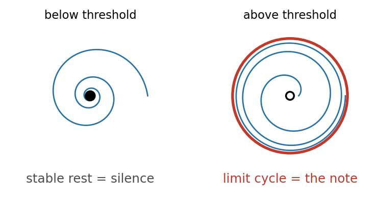
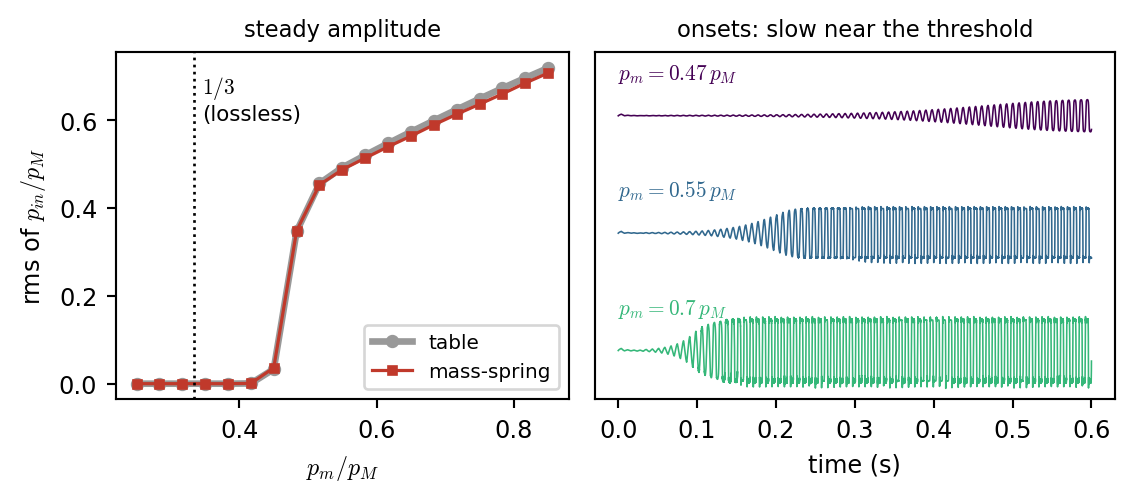
Raise \(p_m\) slowly. Below a threshold the air just flows; above it a limit cycle grows: a Hopf bifurcation (class 13).

  • Lossless bore, quasi-static reed: threshold \(p_m=p_M/3\), where \(U(\Delta p)\) starts falling (negative resistance).
  • With losses: higher (here \(\approx0.43\,p_M\)): the negative resistance must beat the bore loss.
  • Growth rate \(\propto\) distance above threshold: slow onsets near it.

Only a two-way model has a threshold at all: whether a note sounds is decided by the coupling.

Show code
gam = np.linspace(0.25, 0.85, 19); amp = {}
for tab in [True, False]:
    amp[tab] = []
    for g_ in gam:
        bo = Bore(S, **LOSSY); o = play(bo, Reed(bo.Z0, table=tab), g_ * pM, dur=0.6)
        amp[tab].append(np.std(o["pin"][-6000:]) / pM)
fig, axs = plt.subplots(1, 2, figsize=(6.0, 2.7), width_ratios=[1, 1.15])
axs[0].plot(gam, amp[True], "o-", color="0.6", ms=4, lw=2.5, label="table")
axs[0].plot(gam, amp[False], "s-", color=COL["exciter"], ms=3, lw=1.2, label="mass-spring")
axs[0].axvline(1 / 3, color="k", ls=":", lw=1); axs[0].text(0.345, 0.6, "$1/3$\n(lossless)", fontsize=8)
axs[0].set_xlabel("$p_m/p_M$"); axs[0].set_ylabel("rms of $p_{in}/p_M$"); axs[0].legend(fontsize=7.5)
axs[0].set_title("steady amplitude", fontsize=8.5)
for i, g_ in enumerate([0.47, 0.55, 0.7]):
    bo = Bore(S, **LOSSY); o = play(bo, Reed(bo.Z0), g_ * pM, dur=0.6)
    axs[1].plot(np.arange(len(o["pin"])) * k, o["pin"] / pM - 2.4 * i, color=plt.cm.viridis(i / 3), lw=0.6)
    axs[1].text(0.0, -2.4 * i + 0.75, f"$p_m={g_}\\,p_M$", fontsize=8, color=plt.cm.viridis(i / 3))
axs[1].set_ylim(-2.4 * 2 - 1.0, 1.3)
axs[1].set_yticks([]); axs[1].set_xlabel("time (s)"); axs[1].set_title("onsets: slow near the threshold", fontsize=8.5)
plt.tight_layout()
plt.show()

Clarinet vs Saxophone: Same Reed, Different Bore

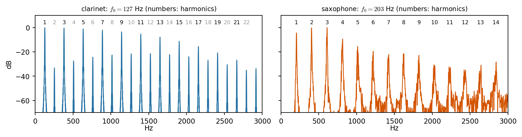
Same reed, same \(p_m=0.5\,p_M\), same length 66.4 cm. One line changes:

S = cylinder(0.664, 0.0074)      # clarinet
S = saxophone()                  # cone (+ mouthpiece)
bo = Bore(S, **LOSSY)
out = play(bo, Reed(bo.Z0), 0.5 * pM)
  • Cylinder: odd harmonics dominate, \(f_0\approx c/4L\).
  • Cone: all harmonics, \(f_0\approx c/2(L+x_0)\): much higher for the same length.
  • The cone is KL steps (a junction per segment); the cylinder needs no junctions at all.

clarinet

saxophone

Show code
fig, axs = plt.subplots(1, 2, figsize=(9.6, 2.6), sharey=True)
for ax, (name, (o, col)) in zip(axs, runs_cs.items()):
    f, Yd = spectrum_db(o["y"]); f0 = f0_of(o["pin"])
    ax.plot(f, Yd, color=col, lw=1)
    for m in range(1, int(2900 / f0) + 1):
        ax.text(m * f0, 3, f"{m}", fontsize=7, ha="center", color="k" if (m % 2 or name == "saxophone") else "0.6")
    ax.set_ylim(-70, 10); ax.set_xlim(0, 3000); ax.set_xlabel("Hz", labelpad=0)
    ax.set_title(f"{name}: $f_0={f0:.0f}$ Hz (numbers: harmonics)", fontsize=8.5)
axs[0].set_ylabel("dB")
plt.tight_layout()
plt.show()

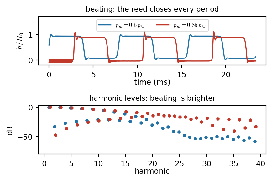
Beating and Squeaks

Show code
fig, axs = plt.subplots(2, 1, figsize=(4.6, 3.1))
sl = slice(int(1.2 * fs), int(1.2 * fs) + int(3 * fs / 128))
for j, (g_, col) in enumerate([(0.5, COL["cyl"]), (0.85, COL["exciter"])]):
    axs[0].plot(1e3 * np.arange(sl.stop - sl.start) * k, beat[g_]["state"][sl] / 4e-4, color=col, lw=1.3, label=f"$p_m={g_}\\,p_M$")
    f, Yd = spectrum_db(beat[g_]["y"]); f0 = f0_of(beat[g_]["pin"]); m = np.arange(1, 40)
    amp = [Yd[np.argmin(np.abs(f - mm * f0))] for mm in m]
    axs[1].plot(m + 0.2 * (j - 0.5), amp, "o", color=col, ms=3)
axs[0].axhline(0, color="k", lw=0.6); axs[0].set_ylabel("$h/H_0$"); axs[0].set_xlabel("time (ms)", labelpad=0)
axs[0].legend(fontsize=7, ncol=2, loc="upper center"); axs[0].set_ylim(-0.2, 1.7); axs[0].set_title("beating: the reed closes every period", fontsize=8.5)
axs[1].set_ylim(-80, 3); axs[1].set_xlabel("harmonic", labelpad=0); axs[1].set_ylabel("dB")
axs[1].set_title("harmonic levels: beating is brighter", fontsize=8.5)
plt.tight_layout()
plt.show()

soft, 0.5 pM

beating, 0.85 pM

Show code
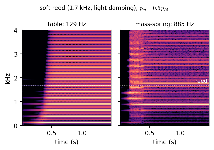
# soft = dict(w0=2 pi 1700, sig=300, same stiffness): a reed resonance close to the high bore modes
fig, axs = plt.subplots(1, 2, figsize=(4.6, 3.1), sharey=True)
for ax, tab in zip(axs, [True, False]):
    show_spec(ax, squeak[tab]["y"], ("table" if tab else "mass-spring") + f": {f0_of(squeak[tab]['pin'], fmax=2000):.0f} Hz", fmax=4)
    ax.axhline(1.7, color="w", ls=":", lw=1); ax.set_xlabel("time (s)")
axs[0].set_ylabel("kHz"); axs[1].text(1.45, 1.8, "reed", color="w", ha="right", fontsize=8)
fig.suptitle("soft reed (1.7 kHz, light damping), $p_m=0.5\\,p_M$", fontsize=8.5)
plt.tight_layout()
plt.show()

table: a normal note

mass-spring: a squeak

Brass: An Outward Striking Lip Valve

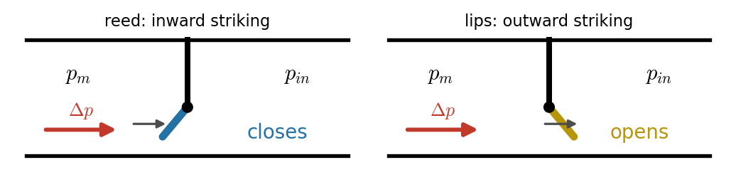
Mouth pressure pushes the lips open (outward striking), the opposite sign of the reed: \[ y''+\frac{\omega_\ell}{Q}y'+\omega_\ell^2(y-y_0)=+\frac{\Delta p}{\mu} \] \[ u=w\,[y]_+\sqrt{\tfrac{2|\Delta p|}{\rho}}\,\operatorname{sgn}\Delta p \] Same scheme, same quadratic per step.

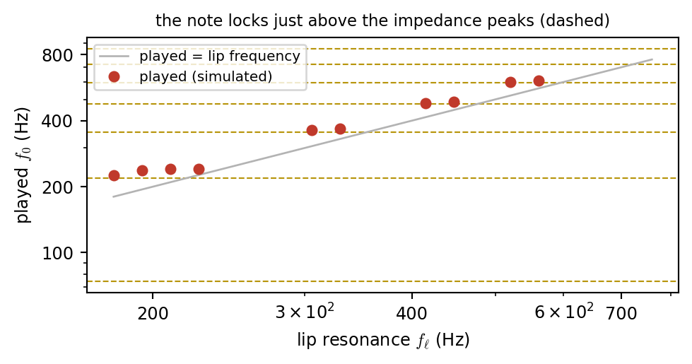
  • Lip resonance \(f_\ell\) near the note, set by the player: no memoryless table possible.
  • The note locks to the impedance peak near \(f_\ell\), slightly above it (outward striking).
  • Tighter lips for higher notes: here \(\mu\propto1/f_\ell\) (a modeling choice to fit to measurements).

Show code
St = trumpet(); f, Z = input_impedance(St, n=1 << 15, **LOSSY)
zpk = peaks_of(f, 20 * np.log10(np.abs(Z)), 900, thr=0)
fl_sweep = np.geomspace(180, 760, 20); played = []
for fl in fl_sweep:
    bo = Bore(St, **LOSSY); o = play(bo, Lips(bo.Z0, fl), 7000.0 * (fl / 200)**0.4, dur=0.4)   # a bit harder up high
    played.append(f0_of(o["pin"]) if np.std(o["pin"][-4000:]) > 100 else np.nan)
fig, ax = plt.subplots(figsize=(5.2, 2.8))
for fp in zpk:
    ax.axhline(fp, color=COL["brass"], lw=0.8, ls="--")
ax.plot(fl_sweep, fl_sweep, color="0.7", lw=1, label="played = lip frequency")
ax.plot(fl_sweep, played, "o", color=COL["exciter"], ms=5, label="played (simulated)")
ax.set_xscale("log"); ax.set_yscale("log"); ax.set_xlabel("lip resonance $f_\\ell$ (Hz)"); ax.set_ylabel("played $f_0$ (Hz)")
ax.set_title("the note locks just above the impedance peaks (dashed)", fontsize=8.5); ax.legend(fontsize=7.5, loc="upper left")
ax.set_yticks([100, 200, 400, 800]); ax.set_yticklabels(["100", "200", "400", "800"])
ax.set_xticks([200, 400, 700]); ax.set_xticklabels(["200", "400", "700"])
plt.tight_layout()
plt.show()

Playing the Harmonic Series

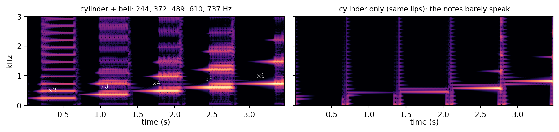
Only the lip tension changes (five settings); the fingering stays.

lips.tune(fl)          # every 0.7 s
  • With the bell: harmonics 2 to 6 of about 123 Hz, the notes of a bugle call.
  • Without it: the same lips find no peak where they ask (the cylinder has only odd ones): the notes barely speak.

with the bell

cylinder only

Show code
fig, axs = plt.subplots(1, 2, figsize=(9.6, 2.3), sharey=True)
for ax, (o, fs_, name) in zip(axs, [(arp_bell, f_bell, "cylinder + bell"), (arp_cyl, f_cyl, "cylinder only (same lips)")]):
    show_spec(ax, o["y"], f"{name}: " + (", ".join(f"{v:.0f}" for v in fs_) + " Hz" if not np.isnan(fs_).any() else "the notes barely speak"), fmax=3)
    ax.set_xlabel("time (s)", labelpad=0)
    base = np.nanmean(np.array(f_bell) / np.arange(2, 7))
for m in range(2, 7):
    axs[0].text(Tn * (m - 1.5), 0.2 + m * base / 1e3, f"$\\times{m}$", color="w", fontsize=8, ha="center")
axs[0].set_ylabel("kHz")
plt.tight_layout()
plt.show()

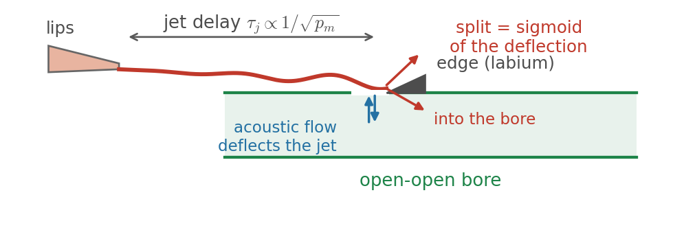
Flute: Jet Delay and a Sigmoid

No valve: an air jet hits a sharp edge (labium).

  1. The acoustic flow at the mouth hole deflects the jet.
  2. The deflection travels along the jet: delay \(\tau_j\propto\ell/U_j\), \(U_j\propto\sqrt{p_m}\).
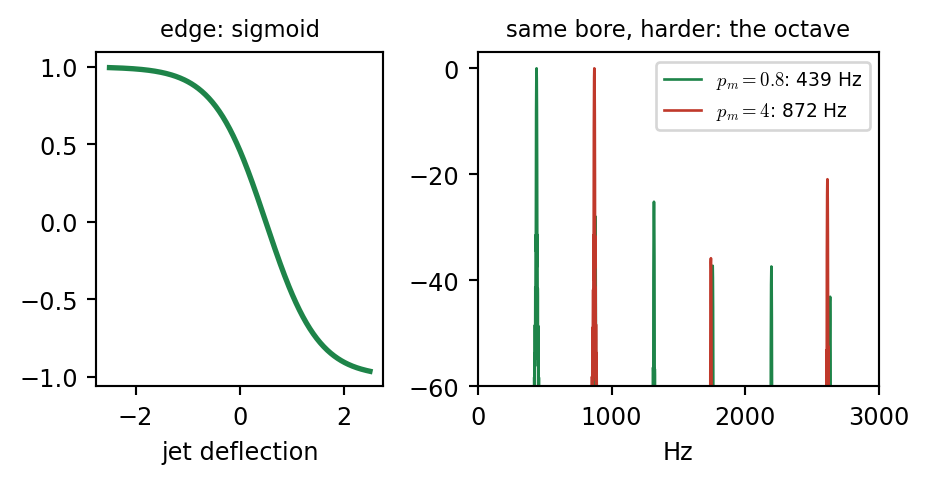
  3. The edge splits the jet: inflow = a sigmoid of the deflection, \(\sqrt{p_m}\tanh(\cdot)\), saturating.
  4. Inflow + noise (turbulence) drives an open-open bore (all harmonics).
d = jet[i - Nj]                          # jet delay
inflow = U * np.tanh(-G * d / U + 0.5)   # edge sigmoid
bore_in = bore_out + inflow

Oscillation needs \(\tau_j\approx T/2\). Blow harder: \(\tau_j\) shrinks, the octave mode fits: overblowing.

soft

overblown

breath + vibrato

Show code
fl_soft = flute(440.0, 0.8, dur=1.6)
fl_hard = flute(440.0, 4.0, dur=1.6)
fl_breath = flute(440.0, 1.0, dur=1.6, noise=0.12, vib=0.04)
for name, y in [("soft", fl_soft), ("hard", fl_hard), ("breathy", fl_breath)]:
    save_wav("flute_" + name, y)
fig, axs = plt.subplots(1, 2, figsize=(4.9, 2.6), width_ratios=[1, 1.4])
xx = np.linspace(-2.5, 2.5, 300)
axs[0].plot(xx, np.tanh(-xx + 0.5), color=COL["flute"], lw=2)
axs[0].set_xlabel("jet deflection"); axs[0].set_title("edge: sigmoid", fontsize=8.5)
for y, col, lab in [(fl_soft, COL["flute"], "$p_m=0.8$"), (fl_hard, COL["exciter"], "$p_m=4$")]:
    f, Yd = spectrum_db(y); axs[1].plot(f, Yd, color=col, lw=1, label=f"{lab}: {f0_of(y):.0f} Hz")
axs[1].set_xlim(0, 3000); axs[1].set_ylim(-60, 3); axs[1].set_xlabel("Hz"); axs[1].legend(fontsize=7)
axs[1].set_title("same bore, harder: the octave", fontsize=8.5)
plt.tight_layout()
plt.show()

Voice: A Parametric Glottal Source

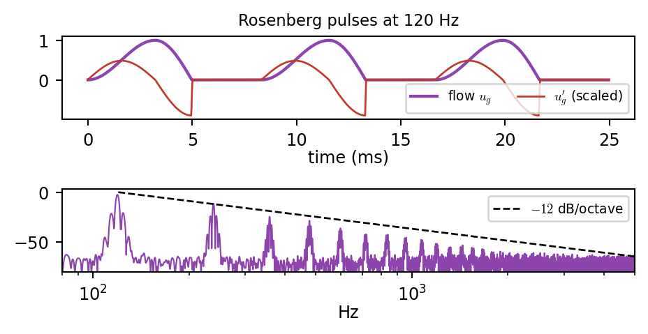
The vocal folds are a self-oscillating valve like the lips (two-mass model of Ishizaka and Flanagan). Yet speech synthesis usually prescribes the flow: source-filter, one-way.

  • The glottis is narrow: its impedance \(\gg Z_0\) of the tract, so the tract barely talks back.
  • Pitch is set by the folds, not by tract resonances.

Rosenberg pulse per period \(T\) (open quotient \(O_q\), skew \(s\)): \[ u_g=\begin{cases}\frac12\big(1-\cos\frac{\pi t}{sO_qT}\big)&\text{opening}\\ \cos\frac{\pi(t-sO_qT)}{2(1-s)O_qT}&\text{closing}\\ 0&\text{closed}\end{cases} \] + vibrato, jitter, breath noise. The LF model draws \(u_g'\) with four parameters; either way, the sharp closure excites the tract.

Show code
ug = glottal_flow(120.0, 1.2)
save_wav("glottis_raw", np.gradient(ug))
fig, axs = plt.subplots(2, 1, figsize=(4.9, 2.6))
ug_clean = glottal_flow(120.0, 1.2, breath=0.0, jitter=0.0, vib=0.0)    # noise free, for the picture
sl = slice(int(0.5 * fs), int(0.5 * fs) + int(3 * fs / 120)); tt = 1e3 * np.arange(sl.stop - sl.start) * k
axs[0].plot(tt, ug_clean[sl], color=COL["voice"], lw=1.6, label="flow $u_g$")
dug = np.gradient(ug_clean[sl]); axs[0].plot(tt, 0.9 * dug / np.abs(dug).max(), color=COL["exciter"], lw=1, label="$u_g'$ (scaled)")
axs[0].set_xlabel("time (ms)", labelpad=0); axs[0].legend(fontsize=7, ncol=2, loc="lower right")
axs[0].set_title("Rosenberg pulses at 120 Hz", fontsize=8.5)
f, Yd = spectrum_db(ug, n=1 << 15)
axs[1].semilogx(f, Yd, color=COL["voice"], lw=0.8)
axs[1].semilogx(f[f > 120], -12 * np.log2(f[f > 120] / 120), "k--", lw=1, label="$-12$ dB/octave")
axs[1].set_xlim(80, 5000); axs[1].set_ylim(-80, 3); axs[1].set_xlabel("Hz", labelpad=0); axs[1].legend(fontsize=7)
plt.tight_layout()
plt.show()

the source alone (radiated, \(u_g'\))

Vowels from Area Functions

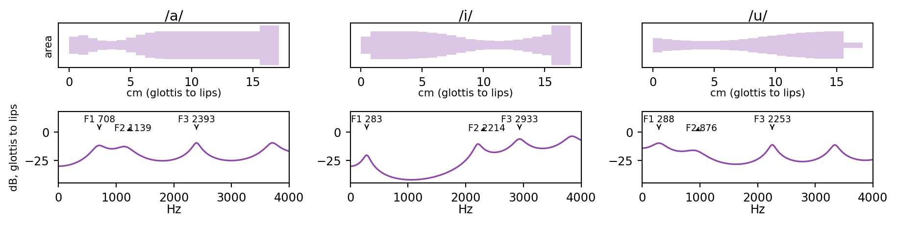
Kelly–Lochbaum tract: 22 segments of 7.8 mm, glottis (reflection \(0.75\)) to lips (lowpass radiation), a little loss per segment for the walls.

Area function, 4 parameters: constriction place \(x_c\), area \(A_c\), width, lip area \(A_\ell\), fitted to textbook formants:

\(F_1\) \(F_2\) shape
/a/ high low back constriction, open lips
/i/ low high front constriction
/u/ low low back constriction, rounded lips

Same glottal source for all three (below).

Show code
# VOWEL = {"a": (0.20, 0.35, 0.12, 8.0), "i": (0.65, 0.35, 0.20, 8.0), "u": (0.25, 0.35, 0.30, 0.15)}
fig, axs = plt.subplots(2, 3, figsize=(9.6, 2.5), height_ratios=[1, 1.6])
axs = axs.T
for row, (v, (A, f, Hd, F)) in enumerate(vowel_tf.items()):
    xs = np.arange(N_TRACT + 1) * dx * 100; r = np.sqrt(np.r_[A, A[-1]] / np.pi) * 100
    axs[row, 0].fill_between(xs, -r, r, step="post", color=COL["voice"], alpha=0.3, lw=0)
    axs[row, 0].set_ylim(-1.8, 1.8); axs[row, 0].set_title(f"/{v}/", fontsize=11, pad=2); axs[row, 0].set_yticks([])
    axs[row, 1].plot(f, Hd, color=COL["voice"], lw=1.2)
    for j, Fj in enumerate(F[:3]):
        axs[row, 1].annotate(f"F{j + 1} {Fj:.0f}", xy=(Fj, 0), xytext=(Fj + (150 if j == 1 else 0), 9 if j != 1 else 1), fontsize=7, ha="center",
                             arrowprops=dict(arrowstyle="->", lw=0.8))
    axs[row, 1].set_xlim(0, 4000); axs[row, 1].set_ylim(-45, 18)
axs[0, 0].set_ylabel("area", fontsize=8); axs[0, 1].set_ylabel("dB, glottis to lips", fontsize=8)
for a_ in axs[:, 0]: a_.set_xlabel("cm (glottis to lips)", labelpad=0, fontsize=8)
for a_ in axs[:, 1]: a_.set_xlabel("Hz", labelpad=0)
plt.tight_layout()
plt.show()

/a/

/i/

/u/

A Diphthong: A Time-Varying Tract

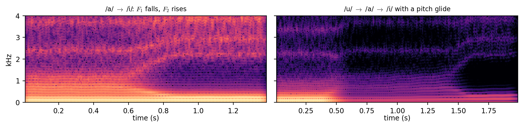
Interpolate the log area between two vowels along a smooth S-curve and update the junctions every sample:

for i in range(n):
    bo.set_S(areas[i])     # time-varying KL
    y[i] = bo.step(rg * bo.b[0] + ug[i])
  • The path and speed of the change matter perceptually: a straight line sounds stiff.
  • Time-varying coefficients can inject energy: the junctions are no longer exactly lossless. Slow changes are safe; fast ones need power-normalized junctions.

/a/ to /i/

/u/ to /a/ to /i/, with a pitch glide

Show code
fig, axs = plt.subplots(1, 2, figsize=(9.6, 2.4), sharey=True)
show_spec(axs[0], y_ai, "/a/ $\\to$ /i/: $F_1$ falls, $F_2$ rises", fmax=4, win=1024)
show_spec(axs[1], y_uai, "/u/ $\\to$ /a/ $\\to$ /i/ with a pitch glide", fmax=4, win=1024)
axs[0].set_ylabel("kHz")
for ax in axs:
    ax.set_xlabel("time (s)", labelpad=0)
plt.tight_layout()
plt.show()

Virtual Tubes

Choosing a Method

Tubes: Waveguide, Finite Differences, or Modal?

digital waveguide finite differences (Webster) modal (impedance peaks)
exactness exact for cylinders and cones small dispersion if \(\lambda<1\) (tiny for tubes) exact modes, if you have them
cost per sample \(O(1)\) for a cylinder (loop filters); \(O(N)\) with KL junctions \(O(N)\) \(O(M)\) modes
varying cross-section KL steps of \(ck\) any \(S(x)\), any grid eigenproblem per shape
time-varying tuning (slide, bend) change a delay (fractional) the grid must change: hard change \(\omega_m\)
nonlinear exciter one scalar per step one scalar per step via impedance, one scalar
extra physics (walls, nonlinear propagation) hard natural linear only
stability \(\lvert H\rvert\le1\): passive by construction CFL + energy always (linear)
2D / 3D mesh: same answer as FD, \(\approx2\times\) cost natural precompute modes

Checklist

  1. Cylinder or cone, real time, pitch bends: waveguide
  2. Measured or designed bore profile, extra physics: finite differences
  1. Measured input impedance, few resonances: modal
  2. 2D or 3D (rooms, plates): finite differences (the mesh loses its edge)

Looking Ahead

Where These Ideas Come Back

  • Sound Effects (next class)
    • time-varying fractional delay: the Doppler shift of a passing car or a siren
    • feedback delay networks: artificial reverberation built from delay lines and a lossless scattering matrix (today’s junctions, generalized)
    • engines and exhausts as driven tubes; whistles and bottles as edge tones (the flute jet); wind as jet noise
    • impacts, scrapes, and rolling: the mallet, friction, and modal bank of classes 16 and 17
  • Projects: Korean winds. The daegeum (a jet with a buzzing membrane, cheong), the piri (double reed, cylinder), the taepyeongso (double reed, cone, metal bell): measure \(S(x)\) and play it.

Recap

Recap on Today’s ILO

  • Digital waveguide: two delay lines of pressure waves
    • loss and radiation lumped into a loop filter (\(|H|\le1\): stable); allpass fractional delay for tuning
    • scattering junctions conserve power; KL tube = Webster FD at \(\lambda=1\); the 2D mesh costs more than FD
  • Bore: impedance peaks are the notes; cylinder odd, cone all, bell = lowpass reflector; toneholes = three-port junctions.
  • Exciters: one scalar per step at the mouthpiece
    • reed: table, or semi-implicit mass-spring with a closed-form root; lips: the same with the opposite sign
    • flute: jet delay + sigmoid; voice: glottal pulse into a KL tract (one-way)
  • Parametric vs coupled: high source impedance or a high resonance allows a table; threshold, beating, squeaks, and lip pitch need two-way coupling.
  • Choose: waveguide for cylinders, cones, real time; FD for arbitrary \(S(x)\) and extra physics; modal for measured impedance.